Discontinuous piecewise linear interpolation in MIPs

I received some questions and feedback due to the post here: http://yetanothermathprogrammingconsultant.blogspot.com/2015/10/piecewise-linear-functions-in-mip-models.html. Here are some “back to basics” notes  on modeling piecewise linear functions. I only look at the easy case: one dimensional only, i.e. y=f(x). This is all simple stuff but it may be useful to show all the different cases in a row. (At least I can now simplify answering a lot of emails by referring to this post).

Continuous, bounded convex case

An example is:

The slope and the intercept can be calculated as:

If the model is convex i.e. if we somehow maximize y using the above curve, then we simple can write:

If we are minimizing y then the curve needs to be sloping up. E.g. in electricity power generation models we often see quadratic cost (to be minimized) as function of output. Of course the sign in the BoundY(s) equation need to be flipped to ≥ in such a case. (Here we have also a possible opportunity to formulate the problem as a MIQP – often we see that a piecewise linear model performs better.)

To emphasize: if we can exploit this convexity, then we don’t need any additional discrete variables.

The fact that we want to bound x between 10 and 45 is easily handled by adding lower and upper bounds to x. This case also deals directly with the unbounded case (see below for a further discussion of this), by just not adding a bound on x.

Continuous, bounded non-convex case

Now assume we don’t have convexity (for instance, we are not maximizing y using the above curve; e.g. because y represents cost). This means we need discrete variables.

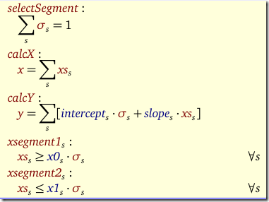
Using binary variables σ_s and additional continuous variables xs_s one could write:

Here xs_s= 0 if x is outside of the selected segment s, and xs_s= x if x is inside this segment s. The selection of a segment is indicated by σ_s=1. In the math above, variables are red and data (constants) are displayed in blue. We see quickly we do not multiply variables by variables and thus this is nicely linear.

This is a little improvement over the discussion in http://yetanothermathprogrammingconsultant.blogspot.com/2015/10/piecewise-linear-functions-in-mip-models.html as we simplified the equation CalcY by doing some data manipulation in advance. In general that is a good idea: it moves complexity away from the equations which are the most difficult to debug. I am a big proponent of keeping the equations as simple as possible.

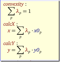
With SOS2 variables λ_p we can do the following. The data requirements are slightly different. We need a table like:

This will allow us to formulate:

Note that we have called here the equation that sums up the λ’s to one: “convexity”. This is the typical name for this equation (even though we are dealing with a non-convex case).

In the following sections we will assume that σ_s∈ {0,1} are binary variables and λ_p are SOS2 variables.

Semi-Continuous, bounded non-convex case

Now assume the data looks like:

This is not so unusual. You get a discount on the (total) price when ordered more than some limit.

The binary variable formulation does not change at all: we can model this directly using the three segments in the table.

The SOS2 variable formulation needs some extra points. Our input for the SOS2 version becomes:

If the curve presents purchasing prices with discounts, this has interesting implications. In this formulation it may be beneficial to order more than you need, just to get the discount. In some models that means modeling some salvage value (can be positive or negative) or even storing it for a future period (adding to inventory).

Typically the solver will not pick a point on a vertical pieces (except for the end points). This is for different reasons. In case we are using the binary variable formulation, it is just not possible to choose those points. In case of the SOS2 formulation, we could end up inside the vertical pieces (not at an end point), but often we minimize or maximize y.

Strange case: discontinuous.

This looks crazy but actually can happen. For instance some types of power generators cannot operate at certain intervals (prohibited zones). A reason could be that amplified vibrations occur at certain operating levels.

The binary variable formulation can deal with this case directly. Unfortunately the SOS2 formulation is not applicable here.

Unbounded case

Now suppose that we don’t have an end point in the last segment (i.e. it just go on forever). Alternatively, we could not have a starting point at the beginning of the first segment. Neither approaches can deal with this case directly. We have to use some possibly large bounds, but in practice that is not a problem. Usually we have some sense of a reasonable lower and upper bound on x.

Simulating SOS2 variables with binary variables

It is possible to mimic the behavior of SOS2 variables using binary variables. To do this we make λ_p positive variables and introduce some binary variables δ_p. Actually the last element of δ_p is not used: it has one element less than λ_p. The SOS2 structure forces that only two consecutive members of λ_p can be non-zero, and this condition we can simulate as follows:

Here we introduces a set p1 (subset of p) with one fewer element than p. The twoeach constraint will make sure only two neigbors of λ_p can be non-zero. The funny syntax is to indicate we do something special for the last equation: the second δ_p is dropped there. This follows the discussion in H. Paul Williams book “Model Building in Mathematical Programming”:

 

Logarithmic number of binary variables

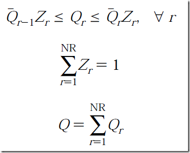
Using a formulation from J. P. Vielma and G. L. Nemhauser. Modeling Disjunctive Constraints with a Logarithmic Number of Binary Variables and Constraints. Mathematical programming, 128(1-2):49-72, 2011 we use a logarithmic number of binary variables. The equations look like:

 

It is needed to use some clever values for L1,L2 (see dissertation by Ernee Kozyre Filho):

and then we end up with something like:

The presence of the expressions 2^t gives a hint that this is related to the power-expansion technique: convert a general integer variable into a series of 0-1 variables.

Note that there are other formulations possible. See e.g. Ming-Hua Lin, John Gunnar Carlsson, Dongdong Ge, Jianming Shi, and Jung-Fa Tsai, “A Review of Piecewise Linearization Methods,” Mathematical Problems in Engineering, 2013

Simple Nash-Cournot equilibrium via EMP

Model OLIGOMCP from the model library is a well-known small Nash-Cournot equilibrium problem, expressed as an MCP:

See also: http://yetanothermathprogrammingconsultant.blogspot.com/2015/03/oligopolistic-producer-behavior-or-why.html and http://amsterdamoptimization.com/pdf/oligopoly.pdf.

This looks like a good example to try the EMP framework and see if we can express the model using the firm’s original maximization problems. The manual is not much of a help here. For this particular type of model the manual (https://www.gams.com/help/topic/gams.doc/solvers/jams/index.html?cp=0_3_23_7#EMP_MOPECs, chapter MOPECs) is not particularly helpful:
”While we do not specify the syntax here for these issues, EMPLIB provides examples that outline how to carry out this matching within GAMS”.

Ok, although a little bit discouraged, lets try anyway. We have 5 firms, each is trying to optimize its profit (revenue – cost) by varying the quantities produced. That is:

using this somewhat complicated cost function. The only way I could make this work was to substitute out Q=∑ q(i) and subsequently p(Q) in this expression, i.e.:

   

Now we can solve:
 

where we need some additional instructions for EMP:

With the PUT statement one could generate this with a loop. From this input deck the EMP tool will differentiate the objectives and form the first order conditions and then call an MCP solver to solve it.

Not sure what is easier: just to formulate the first-order conditions manually or using this EMP tool. Of course there are other good uses for EMP. See for instance: http://www.amazon.com/Complementarity-Modeling-International-Operations-Management/dp/1441961224. And of course there may be better and more elegant ways to write this down that I don’t know about.

Piecewise linear functions in MIP models

Here is a simple case of a piecewise linear function. It shows economies of scale: shipping more leads to lower unit transportation costs.

One way of modeling this is using a set of binary variables indicating in which segment we are:

Then some addition constraints are needed:

and finally we can produce an equation that forms the cost:

When looking at the data:

we can do one simplification: the terms

can be replaced with the coefficients from this table. So a formulation in GAMS could look like:

Usually when I see such structures I first verify if indeed we need binary variables at all (if the cost structure is convex we don’t need them at all). The problem is non-convex so we really need them. The second idea is to use SOS2 variables. Many MIP solvers support SOS2 variables which are designed to these interpolation tasks (see: http://yetanothermathprogrammingconsultant.blogspot.com/2009/06/gams-piecewise-linear-functions-with.html). Let’s see if that simplifies things.

First of all we need to think in points instead of segments. So instead of 4 segments we have now 5 points. We need x and y data (here “q” and “c” data) for these points. Once we calculated the table with the x and y values at the kinks we simply introduce a SOS2 variable λ and we are ready to go:

This is certainly a lot simpler.

This will for sure pay off in larger models. E.g. now I am looking at something like:

Using a proper SOS formulation this can look much less intimidating.

But there is a catch for this model. The SOS2 formulation turns out to be much slower:

Method	Cplex time
Binary variables	Total (root+branch&cut) =    1.95 sec. (488.02 ticks)
SOS2 variables	Total (root+branch&cut) =   79.00 sec. (26865.76 ticks)
Simulate SOS2 variables by binary variables	Total (root+branch&cut) =   21.33 sec. (5435.97 ticks)

The last line is a formulation where we simulate SOS2 variables by binary variables. This is a different approach than the first method. Even that method is more efficient on this model than using SOS2 variables directly.

Note that this is not a Cplex issue per se. Other solvers behave similar. From these experiments and the comments below it really looks like SOS2 variables can cause slower performance, and it may be useful to reformulate with some construct using binary variables.

References:
The model is related to: P. Tsiakis, N. Shah, and C. C. Pantelides, Design of Multi-echelon Supply Chain Networks under Demand Uncertainty, Ind. Eng. Chem. Res. 2001, 40, 3585-3604.
The method where we simulate SOS2 variables using binary variables is documented in: H. Paul Williams, Model Building in Mathematical Programming, Wiley.
See also: http://yetanothermathprogrammingconsultant.blogspot.com/2015/10/discontinuous-piecewise-linear.html
 

Update: additional comments on twitter:

MCP Constraints

When expressing complementarity models it is often needed to “flip” equations around to match the sign of a dual. E.g. a ≥ equation can be paired to a positive dual variable. This sometimes leads to (at least for me) somewhat unnatural formulations such as:

 

or in GAMS:

I really prefer the follow format:

I was unaware of this, but this can actually be done in GAMS by using a – sign in the model statement: this will negate the equation:

model production / FOCproducer.q, −eCapacity.lambda, ePrice.p/;
solve production using mcp;

Finding equidistant Pareto optimal points

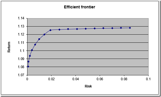
When tracing an efficient frontier sometimes the pictures indicate that points are not very evenly distributed:

In the paper http://www.sciencedirect.com/science/article/pii/S0895717710006424

an interesting algorithm is developed to trace the Pareto frontier with points that are nicely spread out. The idea is to find the next point by adding a distance constraint to the problem. The next point should be a fixed distance from the previous point. Lets try one of the examples in the paper.

The declarations are:

 

Note that the weight λ is now a (nonlinear) variable instead of a parameter.

The example

is implemented as:

The first step is to evaluate the points related to λ=0 and λ=1. I.e. optimize for each objective individually.  (In my experience it is sometimes better not to have the “other” objective just float, but rather have a small weight on that objective. I.e. use λ=0.001 and λ=0.999.)

In line 43, the value for start is kept at zero (which is the default in GAMS; so you don’t see it here – only the nonzero values are shown). In the loop above we made sure we handle obj2 (i.e. λ=1) first and obj1 (λ=0) second. The reason for this is to use the solution for λ=0 as starting point for the loop that traces the frontier. This loop increases λ (forward loop).

Next we calculate the distance between two points γ². We also introduce a constraint that forces the distance between a new point and the last point is γ². I would conjecture that a normalized distance would be more appropriate if the different objectives have different units.

The parameter Δ is used as a simple way to predict a step.

Finally we can execute the main loop:

We set some bounds on the objective variables z (and λ) so we don’t make a step backwards. We estimate the new point using an extremely simple interpolation mechanism. This method is not providing a feasible initial solution for the next point. In the paper it is mentioned they use a smarter estimate that is always feasible. I don’t see immediately how to generate such a starting point.

For the example in question, we get the following picture:

Finally, we can improve on our first picture:

Notes:

• The method in the paper uses much more advanced method to predict the next point in the Homotopy process. For instance they will find estimates that are feasible. My extremely simple method seems to work ok for “easy” problems.
• The paper mentions a backward method (work backwards from λ=1) when the forward method fails. I did not see failures, so I had no need to implement this.

Different but close

In a GAMS model we calculated some numbers. I expected them to be the same. I saw:

OK, small difference. Let’s increase the number of decimals:

No cigar. All right. The difference is beyond the 8th decimal place. Lets have a look in the GDX viewer, which can show things in MAX precision:

Still no luck in viewing the difference between v(c) and v(a),v(b). GDXDUMP?

Export to Excel?

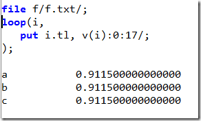
Using PUT?

The PUT statement is limited to 15 decimal places.

We can show some indirect evidence that v(c) actually a little bit larger than v(a) or v(b):

The last bit is different.

Using a C# program writing with d.ToString(“G17’') we finally see the real cause:

Still have not found a easy way (without doing some programming) of showing the numbers v(i) in full precision. Looks like an obvious thing to ask for.