Piecewise linear functions in MIP models

Here is a simple case of a piecewise linear function. It shows economies of scale: shipping more leads to lower unit transportation costs.

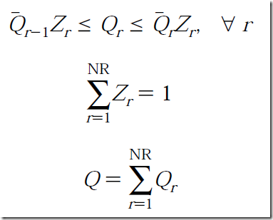
One way of modeling this is using a set of binary variables indicating in which segment we are:

Then some addition constraints are needed:

and finally we can produce an equation that forms the cost:

When looking at the data:

we can do one simplification: the terms

can be replaced with the coefficients from this table. So a formulation in GAMS could look like:

Usually when I see such structures I first verify if indeed we need binary variables at all (if the cost structure is convex we don’t need them at all). The problem is non-convex so we really need them. The second idea is to use SOS2 variables. Many MIP solvers support SOS2 variables which are designed to these interpolation tasks (see: http://yetanothermathprogrammingconsultant.blogspot.com/2009/06/gams-piecewise-linear-functions-with.html). Let’s see if that simplifies things.

First of all we need to think in points instead of segments. So instead of 4 segments we have now 5 points. We need x and y data (here “q” and “c” data) for these points. Once we calculated the table with the x and y values at the kinks we simply introduce a SOS2 variable λ and we are ready to go:

This is certainly a lot simpler.

This will for sure pay off in larger models. E.g. now I am looking at something like:

Using a proper SOS formulation this can look much less intimidating.

But there is a catch for this model. The SOS2 formulation turns out to be much slower:

Method	Cplex time
Binary variables	Total (root+branch&cut) =    1.95 sec. (488.02 ticks)
SOS2 variables	Total (root+branch&cut) =   79.00 sec. (26865.76 ticks)
Simulate SOS2 variables by binary variables	Total (root+branch&cut) =   21.33 sec. (5435.97 ticks)

The last line is a formulation where we simulate SOS2 variables by binary variables. This is a different approach than the first method. Even that method is more efficient on this model than using SOS2 variables directly.

Note that this is not a Cplex issue per se. Other solvers behave similar. From these experiments and the comments below it really looks like SOS2 variables can cause slower performance, and it may be useful to reformulate with some construct using binary variables.

References:
The model is related to: P. Tsiakis, N. Shah, and C. C. Pantelides, Design of Multi-echelon Supply Chain Networks under Demand Uncertainty, Ind. Eng. Chem. Res. 2001, 40, 3585-3604.
The method where we simulate SOS2 variables using binary variables is documented in: H. Paul Williams, Model Building in Mathematical Programming, Wiley.
See also: http://yetanothermathprogrammingconsultant.blogspot.com/2015/10/discontinuous-piecewise-linear.html
 

Update: additional comments on twitter: