Finding equidistant Pareto optimal points

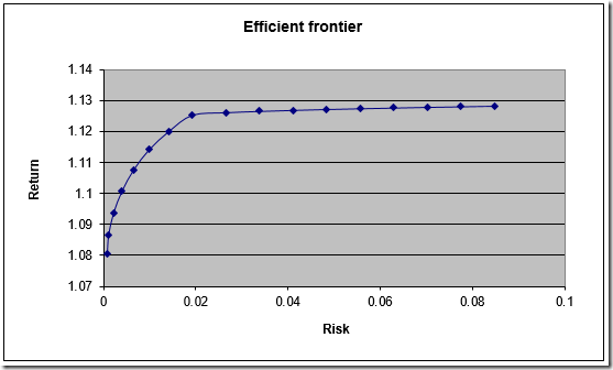
When tracing an efficient frontier sometimes the pictures indicate that points are not very evenly distributed:

In the paper http://www.sciencedirect.com/science/article/pii/S0895717710006424

an interesting algorithm is developed to trace the Pareto frontier with points that are nicely spread out. The idea is to find the next point by adding a distance constraint to the problem. The next point should be a fixed distance from the previous point. Lets try one of the examples in the paper.

The declarations are:

 

Note that the weight λ is now a (nonlinear) variable instead of a parameter.

The example

is implemented as:

The first step is to evaluate the points related to λ=0 and λ=1. I.e. optimize for each objective individually.  (In my experience it is sometimes better not to have the “other” objective just float, but rather have a small weight on that objective. I.e. use λ=0.001 and λ=0.999.)

In line 43, the value for start is kept at zero (which is the default in GAMS; so you don’t see it here – only the nonzero values are shown). In the loop above we made sure we handle obj2 (i.e. λ=1) first and obj1 (λ=0) second. The reason for this is to use the solution for λ=0 as starting point for the loop that traces the frontier. This loop increases λ (forward loop).

Next we calculate the distance between two points γ². We also introduce a constraint that forces the distance between a new point and the last point is γ². I would conjecture that a normalized distance would be more appropriate if the different objectives have different units.

The parameter Δ is used as a simple way to predict a step.

Finally we can execute the main loop:

We set some bounds on the objective variables z (and λ) so we don’t make a step backwards. We estimate the new point using an extremely simple interpolation mechanism. This method is not providing a feasible initial solution for the next point. In the paper it is mentioned they use a smarter estimate that is always feasible. I don’t see immediately how to generate such a starting point.

For the example in question, we get the following picture:

Finally, we can improve on our first picture:

Notes:

• The method in the paper uses much more advanced method to predict the next point in the Homotopy process. For instance they will find estimates that are feasible. My extremely simple method seems to work ok for “easy” problems.
• The paper mentions a backward method (work backwards from λ=1) when the forward method fails. I did not see failures, so I had no need to implement this.