Subset selection in regression

The following is a well-know application of branch-and-bound: select the k best independent variables to include in the regression. Often best means: best residual sum of squares. When we use a slightly different objective we can let the solver decide on k instead of fixing k in advance.

The paper:

 

shows the detailed MIQP model:

We could easily reproduce some of their results in GAMS.

First we load the data into our familiar y and X arrays:

Then we first solve a full OLS to get an estimate of the variance. We need to use the level of the SSQ variable from the solution:

Finally we run the MIQP on the Cp criterion:

Note that the n is a constant, so we could drop it from the objective and find the same optimal solutions. We keep it to make the objective interpretable as the Mallow’s Cp quantity.

Many of the data sets used in the paper contain columns with categorical data. In regression models these are typically handled by a set of dummy variables. When using stepwise regression or a method like MIQP we probably should include (or exclude) a whole block of dummy variables (corresponding to the same categorical variable) instead of considering them individually for inclusion. That makes the MIQP model a bit more complicated to express (but easier to solve).

The housing data set used above had just a single dummy variable. In this case there is no problem. Indeed we can reproduce the results quite easily. From the paper:

We have:

using the formulas:

 

For problems with real categorical data (with more than two levels), we want to adjust the model. In this case we introduce nlevels-1 dummy variables. These dummies belong to the same “block” as they refer to the same categorical variable. We can adapt the MIQP model in two ways:

1. Keep all j binary variables z and add equality constraints for the z’s belonging to the same block.
2. Generate only z(k) binary variables and bound all the beta’s belonging to the same block by the same z(k). I.e. we need to map from beta(j) to z(k).

As the paper notices, when we use  indicator constraints (Cplex, Xpress, SCIP), we could use implications so we don’t have to use a big-M constant

GAMS does not have language facilities to handle this (it allows indicator variables in a Cplex option file, but I feel uncomfortable if an option file – for tolerances and such things – changes the meaning of the model in such a substantial way). Ampl does this better by really having implications in the language.

I don’t really mind using big-M values. As these are essentially bounds on the decision variables, in practice we should be able to come up with a reasonable value.

Note

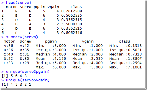
With some of the other data sets I am note sure how the paper arrives at their results. E.g. data set servo:

I.e. we have 4 independent variables, two of which are categorical (motor and screw, both with levels A through E). Pgain and vgain are numerical it looks like. The standard way to handle this in a regression model is to use 4 dummy variables each for the categorical variables motor and screw. Indeed this is what R does:

We see that level A does not generate a dummy variable (instead corresponds to all zeros in the other dummy variables B..E). Pgain and vgain are normal variables. I.e. we end up with a model with a total of p=10 variables (not counting the constant term).

In the paper however we see p=19:

My conjecture is that they did two things differently: the categorical variables are transformed using 5 dummy variables instead of 4; and the variables pgain and vgain are also considered as categorical variables and encoded using 4 and 5 dummies. It is interesting to see how even such a small data set can lead to confusion. How else can we arrive at p=19?

Cplex slides

Slides from ISMP 2015 by CPLEX Optimization Studio engine developers

A number of developers from both engines (CPLEX and CPO) in CPLEX Optimization Studio were in Pittsburgh mid-July for the ISMP 2015 conference. The slides that they presented are available on the IBM Decision Optimization community at https://www.ibm.com/developerworks/community/wikis/home?lang=en#!/wiki/W1a790e980a7d_49c5_963d_2965e5d01401/page/ISMP%202015

These presentations describe how CPO and CPLEX performance were improved in version 12.6.2:
- Handling of symmetries in LP
- Mathematical Programming with indicator constraints
- Failure-directed Search for Constraint-based Scheduling
- Accelerating the Development of Efficient CP Optimizer Models
- Max-Clique cuts
- Advances in CPLEX for Mixed Integer Nonlinear Optimization (12.6.2 is five times faster on MISCOP!)
- Advances in the CPLEX Distributed Solver

MIQP root

Sometimes I see solver logs that makes me wonder… Here is an example:

MIQP Presolve eliminated 1 rows and 1 columns. Reduced MIQP has 3400 rows, 10400 columns, and 2410400 nonzeros. Reduced MIQP has 8000 binaries, 0 generals, 0 SOSs, and 0 indicators. Reduced MIQP objective Q matrix has 2400 nonzeros. Presolve time = 1.77 sec. (674.81 ticks) Probing time = 0.16 sec. (93.32 ticks) Tried aggregator 1 time. Reduced MIQP has 3400 rows, 10400 columns, and 2410400 nonzeros. Reduced MIQP has 8000 binaries, 0 generals, 0 SOSs, and 0 indicators. Reduced MIQP objective Q matrix has 2400 nonzeros. Presolve time = 1.39 sec. (642.45 ticks) Probing time = 0.14 sec. (93.00 ticks) Clique table members: 1000. MIP emphasis: balance optimality and feasibility. MIP search method: dynamic search. Parallel mode: deterministic, using up to 8 threads. Tried aggregator 1 time. No QP presolve or aggregator reductions. Presolve time = 0.25 sec. (125.87 ticks) Parallel mode: using up to 8 threads for barrier. Number of nonzeros in lower triangle of A*A' = 2758800 Using Approximate Minimum Degree ordering Total time for automatic ordering = 1.63 sec. (3083.98 ticks) Summary statistics for Cholesky factor:   Threads                   = 8   Rows in Factor            = 3400   Integer space required    = 10400   Total non-zeros in factor = 3261700   Total FP ops to factor    = 3528593900 Itn      Primal Obj        Dual Obj  Prim Inf Upper Inf  Dual Inf             0  5.5332693e+006 -6.7421398e+006 1.19e+007 1.52e+005 1.77e+005    1  5.5332693e+006  5.4658298e+006 5.88e+004 7.49e+002 8.71e+002    2  5.5332693e+006  5.5328522e+006 2.83e+002 3.61e+000 4.19e+000    3  5.5332693e+006  5.5332673e+006 1.41e+000 1.79e-002 2.08e-002    4  5.5332693e+006  5.5332693e+006 6.99e-003 8.90e-005 1.04e-004    5  5.5332693e+006  5.5332693e+006 3.48e-005 4.43e-007 5.64e-007    6  5.5332693e+006  5.5332693e+006 2.14e-007 2.76e-009 5.25e-008 Barrier time = 5.64 sec. (8857.91 ticks) QP crossover.   Primal and Dual:  Fixing 7000 variables.    Elapsed crossover time = 7.16 sec. (10003.75 ticks, 5945 Superbasics left)      Infeasibility:    Primal 0.00000000e+000     Dual 0.00000000e+000    Elapsed crossover time = 15.31 sec. (28552.30 ticks, 5569 Superbasics left)      Infeasibility:    Primal 0.00000000e+000     Dual 0.00000000e+000    Elapsed crossover time = 23.23 sec. (46704.46 ticks, 5305 Superbasics left)      Infeasibility:    Primal 0.00000000e+000     Dual 0.00000000e+000    Elapsed crossover time = 33.27 sec. (70188.45 ticks, 5054 Superbasics left)      Infeasibility:    Primal 0.00000000e+000     Dual 0.00000000e+000    Elapsed crossover time = 45.64 sec. (98083.66 ticks, 4836 Superbasics left)      Infeasibility:    Primal 0.00000000e+000     Dual 1.39261829e-008    Elapsed crossover time = 57.02 sec. (124653.14 ticks, 4730 Superbasics left)      Infeasibility:    Primal 0.00000000e+000     Dual 4.31355147e-008    Elapsed crossover time = 67.73 sec. (150426.94 ticks, 4649 Superbasics left)      Infeasibility:    Primal 0.00000000e+000     Dual 1.20840923e-007    Elapsed crossover time = 79.16 sec. (176647.52 ticks, 4545 Superbasics left)      Infeasibility:    Primal 0.00000000e+000     Dual 6.72971510e-008    Elapsed crossover time = 90.33 sec. (202789.85 ticks, 4456 Superbasics left)      Infeasibility:    Primal 0.00000000e+000     Dual 9.17043508e-008    Elapsed crossover time = 101.67 sec. (229293.76 ticks, 4372 Superbasics left)      Infeasibility:    Primal 1.47674096e+000     Dual 3.03520210e-007    Elapsed crossover time = 111.36 sec. (251686.98 ticks, 4363 Superbasics left)      Infeasibility:    Primal 1.47681465e+000     Dual 3.78158802e-007    Elapsed crossover time = 120.25 sec. (268368.05 ticks, 4354 Superbasics left)      Infeasibility:    Primal 1.47681459e+000     Dual 3.24780558e-007    Elapsed crossover time = 127.88 sec. (283908.42 ticks, 4240 Superbasics left)      Infeasibility:    Primal 5.93479732e-009     Dual 3.03358320e-007    Elapsed crossover time = 137.27 sec. (304459.09 ticks, 3989 Superbasics left)      Infeasibility:    Primal 6.44471580e-008     Dual 2.18300556e-007    Elapsed crossover time = 149.27 sec. (330999.89 ticks, 3756 Superbasics left)      Infeasibility:    Primal 9.82401907e-006     Dual 6.70703048e-006    Elapsed crossover time = 161.86 sec. (358315.84 ticks, 3719 Superbasics left)      Infeasibility:    Primal 0.00000000e+000     Dual 9.16794306e-007    Elapsed crossover time = 172.38 sec. (383644.53 ticks, 3688 Superbasics left)      Infeasibility:    Primal 0.00000000e+000     Dual 7.28524174e-006    Elapsed crossover time = 183.17 sec. (409268.61 ticks, 3649 Superbasics left)      Infeasibility:    Primal 0.00000000e+000     Dual 1.75125388e-006    Elapsed crossover time = 193.80 sec. (434690.75 ticks, 3616 Superbasics left)      Infeasibility:    Primal 0.00000000e+000     Dual 1.87935366e-005    Elapsed crossover time = 204.61 sec. (461215.00 ticks, 3576 Superbasics left)      Infeasibility:    Primal 0.00000000e+000     Dual 1.03380080e-006    Elapsed crossover time = 215.09 sec. (486417.66 ticks, 3549 Superbasics left)      Infeasibility:    Primal 0.00000000e+000     Dual 1.98637099e-006    Elapsed crossover time = 225.89 sec. (513139.41 ticks, 3510 Superbasics left)      Infeasibility:    Primal 2.10855582e-001     Dual 2.02513729e-006    Elapsed crossover time = 236.05 sec. (535568.96 ticks, 3484 Superbasics left)      Infeasibility:    Primal 6.24493647e-003     Dual 1.52526445e-006 Markowitz threshold set to 0.1    Elapsed crossover time = 248.38 sec. (563321.19 ticks, 3333 Superbasics left)      Infeasibility:    Primal 3.36909296e-003     Dual 4.77023950e-005    Elapsed crossover time = 318.11 sec. (751201.40 ticks, 3333 Superbasics left)      Infeasibility:    Primal 2.12025977e+003     Dual 4.75232446e-005    Elapsed crossover time = 330.94 sec. (789219.13 ticks, 3333 Superbasics left)      Infeasibility:    Primal 9.59407700e-002     Dual 4.77066314e-005    Elapsed crossover time = 343.88 sec. (825357.13 ticks, 3333 Superbasics left)      Infeasibility:    Primal 9.59800219e-002     Dual 6.33971104e-005    Elapsed crossover time = 358.42 sec. (864523.87 ticks, 3333 Superbasics left)      Infeasibility:    Primal 9.34496411e-002     Dual 3.14321933e-005    Elapsed crossover time = 372.47 sec. (904729.79 ticks, 3333 Superbasics left)      Infeasibility:    Primal 9.34088085e-002     Dual 1.75639834e-005    Elapsed crossover time = 388.09 sec. (943680.90 ticks, 3333 Superbasics left)      Infeasibility:    Primal 5.46198930e-002     Dual 9.53896961e-006    Elapsed crossover time = 403.11 sec. (984367.15 ticks, 3333 Superbasics left)      Infeasibility:    Primal 2.90653794e-002     Dual 8.91545915e-005    Elapsed crossover time = 415.58 sec. (1020067.24 ticks, 3333 Superbasics left)      Infeasibility:    Primal 2.89335895e-002     Dual 2.41810067e-005    Elapsed crossover time = 429.14 sec. (1058618.75 ticks, 3333 Superbasics left)      Infeasibility:    Primal 2.84690980e-002     Dual 3.90030436e-005    Elapsed crossover time = 442.63 sec. (1097715.44 ticks, 3333 Superbasics left)      Infeasibility:    Primal 9.78869120e+004     Dual 5.68837444e+003    Elapsed crossover time = 456.14 sec. (1134758.50 ticks, 3333 Superbasics left)      Infeasibility:    Primal 4.67225351e+004     Dual 5.77386458e+003    Elapsed crossover time = 470.00 sec. (1172495.60 ticks, 3333 Superbasics left)      Infeasibility:    Primal 5.53826983e+004     Dual 6.83817634e+003    Elapsed crossover time = 486.74 sec. (1215601.97 ticks, 3333 Superbasics left)      Infeasibility:    Primal 9.41979528e+004     Dual 1.17608258e+004    Elapsed crossover time = 500.95 sec. (1251898.93 ticks, 3333 Superbasics left)      Infeasibility:    Primal 2.39769777e+005     Dual 3.00622953e+004    Elapsed crossover time = 515.22 sec. (1289115.60 ticks, 3333 Superbasics left)      Infeasibility:    Primal 4.88061211e+003     Dual 7.54748835e+002    Elapsed crossover time = 529.25 sec. (1327038.38 ticks, 3333 Superbasics left)      Infeasibility:    Primal 4.88061211e+003     Dual 7.54748835e+002    Elapsed crossover time = 542.24 sec. (1357677.33 ticks, 3333 Superbasics left)      Infeasibility:    Primal 3.65324988e+003     Dual 1.26132745e+003    Elapsed crossover time = 552.99 sec. (1386459.18 ticks, 3333 Superbasics left)      Infeasibility:    Primal 3.65324988e+003     Dual 1.26132745e+003    Elapsed crossover time = 565.88 sec. (1418048.64 ticks, 3333 Superbasics left)      Infeasibility:    Primal 2.16480240e+003     Dual 1.91691257e+003    Elapsed crossover time = 579.27 sec. (1453911.63 ticks, 3333 Superbasics left)      Infeasibility:    Primal 2.16353933e+003     Dual 1.91678103e+003    Elapsed crossover time = 588.53 sec. (1480497.42 ticks, 3333 Superbasics left)      Infeasibility:    Primal 2.16353933e+003     Dual 1.91678103e+003    Elapsed crossover time = 597.89 sec. (1504777.31 ticks, 3333 Superbasics left)      Infeasibility:    Primal 1.90094988e+003     Dual 1.14836471e+004    Elapsed crossover time = 604.97 sec. (1521009.73 ticks, 3333 Superbasics left)      Infeasibility:    Primal 1.90129768e+003     Dual 1.15904573e+004    Elapsed crossover time = 611.22 sec. (1536795.42 ticks, 3333 Superbasics left)      Infeasibility:    Primal 1.90129768e+003     Dual 1.15904573e+004    Elapsed crossover time = 616.67 sec. (1551877.10 ticks, 3333 Superbasics left)      Infeasibility:    Primal 1.90773276e+003     Dual 1.17815647e+004    Elapsed crossover time = 622.81 sec. (1567277.44 ticks, 3333 Superbasics left)      Infeasibility:    Primal 1.90773276e+003     Dual 1.17815647e+004    Elapsed crossover time = 627.38 sec. (1580302.78 ticks, 3333 Superbasics left)      Infeasibility:    Primal 1.89426710e+003     Dual 1.07900064e+004    Elapsed crossover time = 631.66 sec. (1591985.82 ticks, 3333 Superbasics left)      Infeasibility:    Primal 1.87985719e+003     Dual 1.00576739e+004    Elapsed crossover time = 637.89 sec. (1609258.08 ticks, 3333 Superbasics left)      Infeasibility:    Primal 1.90150876e+003     Dual 7.31013617e+003    Elapsed crossover time = 642.83 sec. (1622767.95 ticks, 3333 Superbasics left)      Infeasibility:    Primal 1.90150876e+003     Dual 7.31013617e+003    Elapsed crossover time = 647.22 sec. (1635731.36 ticks, 3333 Superbasics left)      Infeasibility:    Primal 1.86842002e+003     Dual 7.13853235e+003    Elapsed crossover time = 652.58 sec. (1650655.52 ticks, 3333 Superbasics left)      Infeasibility:    Primal 1.84100817e+003     Dual 1.21837103e+004    Elapsed crossover time = 657.20 sec. (1663498.01 ticks, 3333 Superbasics left)      Infeasibility:    Primal 1.76000240e+003     Dual 2.90792871e+004    Elapsed crossover time = 662.86 sec. (1679982.33 ticks, 3333 Superbasics left)      Infeasibility:    Primal 1.85701960e+003     Dual 7.13495764e+003    Elapsed crossover time = 667.89 sec. (1691903.10 ticks, 3333 Superbasics left)      Infeasibility:    Primal 1.96317658e+004     Dual 5.10543645e+005    Elapsed crossover time = 671.80 sec. (1703072.56 ticks, 3333 Superbasics left)      Infeasibility:    Primal 4.03036288e+004     Dual 1.07718950e+006    Elapsed crossover time = 675.69 sec. (1714438.25 ticks, 3333 Superbasics left)      Infeasibility:    Primal 2.16603817e+003     Dual 2.76079763e+004    Elapsed crossover time = 680.95 sec. (1728011.91 ticks, 3333 Superbasics left)      Infeasibility:    Primal 2.41650804e+003     Dual 2.61412656e+004    Elapsed crossover time = 684.88 sec. (1738262.56 ticks, 3333 Superbasics left)      Infeasibility:    Primal 2.92877479e+003     Dual 4.13609774e+004    Elapsed crossover time = 689.19 sec. (1748946.49 ticks, 3333 Superbasics left)      Infeasibility:    Primal 1.25701941e+004     Dual 1.56358766e+005    Elapsed crossover time = 694.44 sec. (1761372.46 ticks, 3333 Superbasics left)      Infeasibility:    Primal 2.31800356e+003     Dual 1.89475266e+004    Elapsed crossover time = 699.81 sec. (1772146.05 ticks, 3333 Superbasics left)      Infeasibility:    Primal 6.42620370e+003     Dual 5.49984245e+004    Elapsed crossover time = 705.53 sec. (1782843.13 ticks, 3333 Superbasics left)      Infeasibility:    Primal 2.15767429e+006     Dual 1.75141610e+007    Elapsed crossover time = 711.47 sec. (1793058.87 ticks, 3333 Superbasics left)      Infeasibility:    Primal 2.21269742e+003     Dual 8.03297651e+004    Elapsed crossover time = 718.33 sec. (1803421.24 ticks, 3333 Superbasics left)      Infeasibility:    Primal 7.53001991e+005     Dual 2.93476689e+007    Elapsed crossover time = 725.44 sec. (1813741.70 ticks, 3332 Superbasics left)      Infeasibility:    Primal 1.24805125e+004     Dual 1.29957987e+006    Elapsed crossover time = 732.19 sec. (1823771.99 ticks, 3332 Superbasics left)      Infeasibility:    Primal 3.17114125e+003     Dual 4.33555604e+005    Elapsed crossover time = 738.59 sec. (1833802.22 ticks, 3332 Superbasics left)      Infeasibility:    Primal 6.00998749e+006     Dual 1.02118829e+009    Elapsed crossover time = 745.03 sec. (1843805.29 ticks, 3332 Superbasics left)      Infeasibility:    Primal 3.79317034e+006     Dual 6.44532210e+008    Elapsed crossover time = 751.81 sec. (1854167.14 ticks, 3332 Superbasics left)      Infeasibility:    Primal 5.03251939e+005     Dual 2.28553099e+008    Elapsed crossover time = 758.20 sec. (1864411.09 ticks, 3332 Superbasics left)      Infeasibility:    Primal 3.03520837e+006     Dual 8.01584368e+008    Elapsed crossover time = 764.67 sec. (1874969.68 ticks, 3332 Superbasics left)      Infeasibility:    Primal 4.65210530e+006     Dual 4.55334749e+009    Elapsed crossover time = 770.52 sec. (1885177.76 ticks, 3332 Superbasics left)      Infeasibility:    Primal 4.97860595e+007     Dual 8.99304928e+010    Elapsed crossover time = 776.05 sec. (1895242.21 ticks, 3332 Superbasics left)      Infeasibility:    Primal 3.99168883e+007     Dual 3.21266821e+011   Primal:  Pushed 48, exchanged 4653.   Dual  :  Pushed 0, exchanged 4691. Warning: Crossover terminates with a singular basis.

I.e. 5 seconds to solve the relaxed qp and then spending 775 seconds in the crossover (without a good result)!

It is good to see that there is progress in this area (quadratic related optimization). E.g. from a recent presentation:

(http://www.slideshare.net/IBMOptimization/euro-2015-nodet). In general my feeling is that quadratic solvers are not as mature as linear solvers, and occasional show erratic behavior. As I see typically difficult models (for easy ones users don’t need my help), I encounter issues like these more than I care for.

Calculating the Bacon number: a shortest path network

The Bacon number measures how far an actor is removed from Kevin Bacon in terms of playing in the same movie. I received a data set with actors and movies. As this problem can be written as standard network model we can easily solve this with an LP solver.

Networks are often an important part of math programming models. We see them in supply chain models, in models dealing with electricity grids, regional trade flows, transportation etc. Not all users find this easy to model. Here some notes:

• In this model we moved some of the complexity into the data manipulation step. As a result the equations are very simple. Complex equations are much more difficult to debug.
• The sparse vector b only has two elements. In GAMS only the non-zero elements are stored so this is quite efficient.
• Sometimes users use three different type of flow balance equations. I prefer a single equation block with source and sink modeled via this b vector.
• I have seen implementations where movies are also part of the network. In this case I only have “actor-nodes”, which makes the network smaller.
• The set arcs plays an important role in the topology of the network.
• The network is sparse: many arcs do not exist. This is beneficial for the LP solver.
• I sometimes see users creating a large cost to indicate a link can not be chosen. I think it is often much better to exclude such links from the set arcs.
• In this case we have modeled a directed graph. I prefer to use directed links as the results are easier to interpret and the modeling is much more straightforward. When using undirected arcs we need to look at the sign of the flows. 
• The Bacon number is the length of the shortest path where each link has a unit length. Not each optimal solution is unique. This is a pure network model; in practice we often see more complex models with a network component.
• For pure networks we can easily form and solve the dual. I prefer to stay closer to the problem with a more intuitive primal formulation.
• Of course Google can find these numbers for you:
  

monotonic transformations

From: lp_solve@yahoogroups.com
To: lp_solve@yahoogroups.com
Date: Thu, 9 Jul 2015 00:32:47 -0700
Subject: [lp_solve] C# to set the object with the form of square

Could LP set the object in a form of square? Just like this :
min: Q^2

If we have Q≥0 then just use MIN Q. We can apply a monotonic function. I have used this trick a lot in the context of minimizing distances. Instead of

we can keep things quadratic by using

This got rid of a nasty square root and this allowed us use quadratic solvers.

Back to the original problem where we want to remove a square. What if we don’t know in advance that Q≥0? Then we can solve two problems:

and pick the best one.

The suggested solution in the thread: “Have a look into piecewise linear approximations” is at least much overkill.

Accessing GAMS GDX files as database tables

GAMS GDX files are accessed via an a low-level API. One way to make GDX files more appealing to programmers is to use a higher-level API. One possibility is to use an SQL API. This allows us to use  a very familiar API, Also we can apply certain transformations directly at the SQL level to make data more useful for the host application. Note that we don’t import GDX data into a database here, but rather access GDX data directly through an SQL engine.

GAMS data can often be mapped to SQL tables in a straightforward manner:

Interestingly, we have used SQLite and their virtual table mechanism (https://www.sqlite.org/vtab.html) for this exercise. SQLite allows to store strings in any column. In that sense it is more like Excel. This flexible mechanism would allow us to store normal numbers as DOUBLE values and those GAMS related special values as TEXT.

Here is a small example:

Results from prototype implementation:

Note that the GAMS code to get this result is more complicated:

Sorting is another area where SQL is much more convenient than GAMS code. Being able to do things where GAMS lacks expressiveness seems like a win to me.

With this SQL layer there are many new possibilities, such as:

• Use GDX files through ODBC allowing many applications to access GDX data without any programming effort
• The same ODBC layer also allows access to GDX data from many programming languages using a standard, well-known API
• Use GDX files through LINQ queries from .Net applications
• Writing GDX files (but there are severe restrictions in the GDX API in this respect – e.g. one symbol at the time and only one batch of inserts, no updates).

Of course the price we pay is performance. In many cases we need to do a full table scan. For extremely large data sets, programming directly against the GDX API is still the best solution. Note that in some cases we can increase performance by importing data into a local data base using a SELECT … INTO, after which we can add some clever SQL indices.  

Multinomial probability derivation

For an optimization problem related to media planning I needed to evaluate the probability that a multinomial variate assume the value zero. This can be written as:

However it was suggested to use the following expression:

I did not see immediately that these things are approximately the same. With a little bit of effort:

where the last step is based on a Taylor approximation:

To be precise:

This approximation in evaluating the reach for some advertisement plans seem to work very well.

GAMS limits on labels

In GAMS strings are used for indexing. E.g.

There is a very tight limit on the length of these labels: 63 characters!! This sounds like a strange limit, and it surely is. It is also way too small to handle many datasets from sources like databases and spreadsheets. As these labels are really data, and come form different data sources we do not always have control over their format. That means sometimes we cannot read (otherwise correct) data. In those cases we have to spend time and effort to devise workarounds. In some cases we can truncate strings (e.g. using LEFT(column_name,63) in an SQL query). Note that this would still make it more difficult to put the solution back into the database. And in some cases we see that truncation will not yield unique names. This happens when some names are only different after 63 characters. In that case we have a real problem. This is not just a theoretical possibility: I received just last week a spreadsheet that showed this issue. In another application based on a MySQL database, I am forced to use ugly short codes instead of long descriptive names for the same reason.

So we can conclude: the 63 character limit is just inadequate. A tool like GAMS is supposed to help making a modeler more productive, and this limit is really not doing that. What should the limit be? I have heard that the GAMS people are pondering to make this limit 255 characters. This is much better, but I would argue that this is still the wrong approach. With software we typically have a trade-off between development cost and effort and productivity gains for the end-user. COTS (Commercial Off-the-shelf) software often tips the scale in favor of the user: there are just many users. I.e. making things easy for the programmer should be a secondary concern. So I would argue to spend a little more effort by the developer to implement a really long label functionality (e.g. up to 2^31-1).

If we look at the table below, we see what kind of limits are imposed by other software (often used as data source for GAMS models):

Software	Limits	Unicode
Excel	32,767	Yes
SQL Server	char(n): 8,000 varchar(n): 8,000 varchar(max): 2^31-1 text: 2^31-1	nchar, nvarchar, ntext
Oracle	char(n): 2,000 varchar(n), varchar2(n): 4,000	nchar, nvarchar
DB2	char(n): 254 varchar(n): 32,672 CLOB: 2^31-1	Yes
MySQL	char(n): 255 varchar(n): 65,535 tinytext: 255 text; 65,535 mediumtext: 2^16-1 longtext: 2^32-1	Yes
MS Access	text: 255 memo: 65,536	Yes
SQLite	text: 2^31-1	Yes

Unicode or UTF-8 support would be required to read tables like:

Most modern software can handle this kind of data. The table above is from Excel. A modern editor like Notepad++ or Atom can also handle this:

 

There is an argument to be made to allow Unicode labels. Not as simple as pure ascii though; here is a unicode table:

(http://farmdev.com/talks/unicode/)

Microsoft has ownership of R?

From an (ex-) intellectual property lawyer at Adobe (http://www.infoworld.com/article/2940508/big-data/hey-microsoft-a-rewrite-of-the-r-language-is-a-silly-idea.html): 

“Microsoft, unlike Tibco, can claim ownership of the underlying R code. By buying Revolution Analytics, Microsoft gained that ownership”

I was worried. But luckily it looks like this was misinformation. The new version of the article says:

“Correction: An earlier version of this article incorrectly assumed that Microsoft acquired the rights to R Project from Revolution Analytics. As Revolution Analytics chief community officer David Smith has since stressed, "R is owned by the R Foundation," not Microsoft.”

MPS pictures

http://blogs.sas.com/content/operations/2015/06/25/finding-the-beauty-in-optimization-models-visualizing-mps-data-sets/

Somehow I find these pictures not very helpful in my modeling work. One reason is that problems that don’t display this structure may be very well decomposable. The ordering of rows and columns is very important to detect this structure visually. E.g. I often use a time index t as last index in my variables and equations. As the last index runs the fastest, that will not give these nice pictures. Also modeling systems will likely export all variables x() before y() – i.e. ordered by variable (equation) name. In general you will need to reorder rows and columns to make these pictures meaningful.