Simple Nash-Cournot equilibrium via EMP

Model OLIGOMCP from the model library is a well-known small Nash-Cournot equilibrium problem, expressed as an MCP:

See also: http://yetanothermathprogrammingconsultant.blogspot.com/2015/03/oligopolistic-producer-behavior-or-why.html and http://amsterdamoptimization.com/pdf/oligopoly.pdf.

This looks like a good example to try the EMP framework and see if we can express the model using the firm’s original maximization problems. The manual is not much of a help here. For this particular type of model the manual (https://www.gams.com/help/topic/gams.doc/solvers/jams/index.html?cp=0_3_23_7#EMP_MOPECs, chapter MOPECs) is not particularly helpful:
”While we do not specify the syntax here for these issues, EMPLIB provides examples that outline how to carry out this matching within GAMS”.

Ok, although a little bit discouraged, lets try anyway. We have 5 firms, each is trying to optimize its profit (revenue – cost) by varying the quantities produced. That is:

using this somewhat complicated cost function. The only way I could make this work was to substitute out Q=∑ q(i) and subsequently p(Q) in this expression, i.e.:

   

Now we can solve:
 

where we need some additional instructions for EMP:

With the PUT statement one could generate this with a loop. From this input deck the EMP tool will differentiate the objectives and form the first order conditions and then call an MCP solver to solve it.

Not sure what is easier: just to formulate the first-order conditions manually or using this EMP tool. Of course there are other good uses for EMP. See for instance: http://www.amazon.com/Complementarity-Modeling-International-Operations-Management/dp/1441961224. And of course there may be better and more elegant ways to write this down that I don’t know about.

Piecewise linear functions in MIP models

Here is a simple case of a piecewise linear function. It shows economies of scale: shipping more leads to lower unit transportation costs.

One way of modeling this is using a set of binary variables indicating in which segment we are:

Then some addition constraints are needed:

and finally we can produce an equation that forms the cost:

When looking at the data:

we can do one simplification: the terms

can be replaced with the coefficients from this table. So a formulation in GAMS could look like:

Usually when I see such structures I first verify if indeed we need binary variables at all (if the cost structure is convex we don’t need them at all). The problem is non-convex so we really need them. The second idea is to use SOS2 variables. Many MIP solvers support SOS2 variables which are designed to these interpolation tasks (see: http://yetanothermathprogrammingconsultant.blogspot.com/2009/06/gams-piecewise-linear-functions-with.html). Let’s see if that simplifies things.

First of all we need to think in points instead of segments. So instead of 4 segments we have now 5 points. We need x and y data (here “q” and “c” data) for these points. Once we calculated the table with the x and y values at the kinks we simply introduce a SOS2 variable λ and we are ready to go:

This is certainly a lot simpler.

This will for sure pay off in larger models. E.g. now I am looking at something like:

Using a proper SOS formulation this can look much less intimidating.

But there is a catch for this model. The SOS2 formulation turns out to be much slower:

Method	Cplex time
Binary variables	Total (root+branch&cut) =    1.95 sec. (488.02 ticks)
SOS2 variables	Total (root+branch&cut) =   79.00 sec. (26865.76 ticks)
Simulate SOS2 variables by binary variables	Total (root+branch&cut) =   21.33 sec. (5435.97 ticks)

The last line is a formulation where we simulate SOS2 variables by binary variables. This is a different approach than the first method. Even that method is more efficient on this model than using SOS2 variables directly.

Note that this is not a Cplex issue per se. Other solvers behave similar. From these experiments and the comments below it really looks like SOS2 variables can cause slower performance, and it may be useful to reformulate with some construct using binary variables.

References:
The model is related to: P. Tsiakis, N. Shah, and C. C. Pantelides, Design of Multi-echelon Supply Chain Networks under Demand Uncertainty, Ind. Eng. Chem. Res. 2001, 40, 3585-3604.
The method where we simulate SOS2 variables using binary variables is documented in: H. Paul Williams, Model Building in Mathematical Programming, Wiley.
See also: http://yetanothermathprogrammingconsultant.blogspot.com/2015/10/discontinuous-piecewise-linear.html
 

Update: additional comments on twitter:

MCP Constraints

When expressing complementarity models it is often needed to “flip” equations around to match the sign of a dual. E.g. a ≥ equation can be paired to a positive dual variable. This sometimes leads to (at least for me) somewhat unnatural formulations such as:

 

or in GAMS:

I really prefer the follow format:

I was unaware of this, but this can actually be done in GAMS by using a – sign in the model statement: this will negate the equation:

model production / FOCproducer.q, −eCapacity.lambda, ePrice.p/;
solve production using mcp;

Finding equidistant Pareto optimal points

When tracing an efficient frontier sometimes the pictures indicate that points are not very evenly distributed:

In the paper http://www.sciencedirect.com/science/article/pii/S0895717710006424

an interesting algorithm is developed to trace the Pareto frontier with points that are nicely spread out. The idea is to find the next point by adding a distance constraint to the problem. The next point should be a fixed distance from the previous point. Lets try one of the examples in the paper.

The declarations are:

 

Note that the weight λ is now a (nonlinear) variable instead of a parameter.

The example

is implemented as:

The first step is to evaluate the points related to λ=0 and λ=1. I.e. optimize for each objective individually.  (In my experience it is sometimes better not to have the “other” objective just float, but rather have a small weight on that objective. I.e. use λ=0.001 and λ=0.999.)

In line 43, the value for start is kept at zero (which is the default in GAMS; so you don’t see it here – only the nonzero values are shown). In the loop above we made sure we handle obj2 (i.e. λ=1) first and obj1 (λ=0) second. The reason for this is to use the solution for λ=0 as starting point for the loop that traces the frontier. This loop increases λ (forward loop).

Next we calculate the distance between two points γ². We also introduce a constraint that forces the distance between a new point and the last point is γ². I would conjecture that a normalized distance would be more appropriate if the different objectives have different units.

The parameter Δ is used as a simple way to predict a step.

Finally we can execute the main loop:

We set some bounds on the objective variables z (and λ) so we don’t make a step backwards. We estimate the new point using an extremely simple interpolation mechanism. This method is not providing a feasible initial solution for the next point. In the paper it is mentioned they use a smarter estimate that is always feasible. I don’t see immediately how to generate such a starting point.

For the example in question, we get the following picture:

Finally, we can improve on our first picture:

Notes:

• The method in the paper uses much more advanced method to predict the next point in the Homotopy process. For instance they will find estimates that are feasible. My extremely simple method seems to work ok for “easy” problems.
• The paper mentions a backward method (work backwards from λ=1) when the forward method fails. I did not see failures, so I had no need to implement this.

Different but close

In a GAMS model we calculated some numbers. I expected them to be the same. I saw:

OK, small difference. Let’s increase the number of decimals:

No cigar. All right. The difference is beyond the 8th decimal place. Lets have a look in the GDX viewer, which can show things in MAX precision:

Still no luck in viewing the difference between v(c) and v(a),v(b). GDXDUMP?

Export to Excel?

Using PUT?

The PUT statement is limited to 15 decimal places.

We can show some indirect evidence that v(c) actually a little bit larger than v(a) or v(b):

The last bit is different.

Using a C# program writing with d.ToString(“G17’') we finally see the real cause:

Still have not found a easy way (without doing some programming) of showing the numbers v(i) in full precision. Looks like an obvious thing to ask for.

SQL as optimization language?

https://nathanbrixius.wordpress.com/2015/09/24/sql-as-an-optimization-modeling-language/

Of course the answer is no. SQL is good to deal with data tables but trying to shoehorn optimization models into SQL looks to me like using the wrong tool.

There have been more attempts in this direction:

http://pubsonline.informs.org/doi/abs/10.1287/opre.48.6.846.12388

To me it feels a bit like writing a Basic interpreter in TeX (https://www.tug.org/TUGboat/tb11-3/tb29greene.pdf), interesting from a theoretical point of view but of limited use in practice.

Using relational databases to do some data wrangling is of course a different thing. Many or even most practical models have a significant amount of data manipulation. E.g. often the pure model equations take less than 10% in a real GAMS model. The interesting thing about using a relational database to store model is that we are more flexible: we have more freedom into deciding where to do certain data steps. We can do them in SQL or in the modeling language. Especially when looking at the skill set of developers, it may be a good idea to offload data manipulation to the SQL layer (there are more developers familiar with SQL than with GAMS or AMPL). As the data manipulation part of a modeling exercise is often the most significant part, this division of labor can pay off. 

Of course not all data stuff can be done conveniently in SQL. Currently I am working on a project where just to get some good big-M values needed in some MIP models, we actually solve a series of optimization models. Data steps requiring optimization is not that unusual: e.g. in economic models we often use some matrix balancing to get the data in shape.

Writing the optimization model itself in SQL, in my mind, has little value. For simple, small models it has no particular advantage above a Lindo style, LP file input. For large, more complex models it just will not work. A language is meant to express the problem at hand somewhat conveniently and also should help you to reason and think about the problem. I don’t believe SQL is doing a good job here.

Update: a more detailed list of arguments in favor of SQL: https://nathanbrixius.wordpress.com/2015/10/01/optimization-using-sql-not-crazy/

Linearizations in a Land-Use Planning Model

There are often multiple ways to formulate a problem. With a modeling language it is easy to try out quickly different formulations. This can have a significant effect on the performance of the model.

Problem description

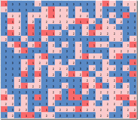
Assuming a grid of cells (plots) we want to assign plots to a certain land use. Each plot has different development cost for different cells. This is much like an assignment problem. Each plot is assigned to a single land-use type and the total area to be assigned to each land-use type is given. Below is an example of a solution if we minimize the total cost using random cost coefficients on a 20 x 20 grid with three land-use types:

This assignment is in practice not very good: we also require some clustering or compactness. Here is a solution where we use a composite objective function with a cost component and a compactness component:

Problem set up

This problem requires just a few sets and some data. The cost data is randomly generated.

MINLP/MIQCP Model

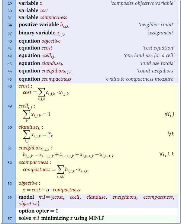
The MINLP model for this problem can look like:

The interesting part is how the compactness is expressed. Basically a plot gets more weight if the cell and its neighbors have the same land use type. The equations eneighbors and ecompactness take care of this. Unfortunately in equation ecompactness we multiply two variables resulting in a MINLP model. Looking at the nature of the non-linearities we can see they are quadratic. This makes it possible to use solvers like Cplex and Gurobi to solve this.

Linearization I

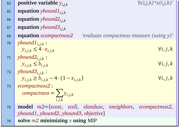
In the paper by Aerts e.a. the following linearization is suggested:

In the paper the variable b is substituted out, but I rather keep it in the model.

Linearization II

Here I propose a different linearization. Instead of linearizing the expression

 

it may be useful to linearize the components:

 

We can do this as follows:

We added some complexity here: the offset parameter indicates the lead (+1) and lags (-1) on the indices i and j. Once we have this offset parameter correctly set up we can deal with these four different binary multiplications in one swoop, using the familiar:

Linearization III

When we take the objective into account, we can see we actually can drop equation gambound3 from the last model. The reason is that the model will automatically try to push the values for Γ upwards (we are minimizing –Γ). So our next version of the model would be:

Linearization IV

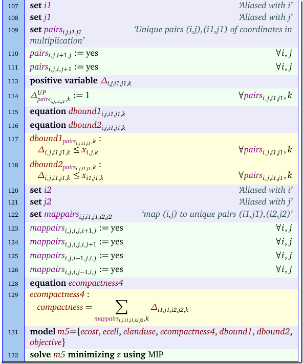
There is further improvement possible by considering that we are repeating some binary multiplications. When considering cell (2,2) we use x(2,3)*x(2,2) and when considering cell (2,3) we look at x(2,2)*x(2,3). However these are the same. Keeping track which pairs we already considered is an interesting exercise.

Here is one approach where we use extra sets to do some bookkeeping.

Performance

In some cases the last formulation is much better (all timings in seconds using one thread):

Model	Solver	Objective	Solve Time	Nodes	Equations/Variables	Notes
MIQCP	Gurobi	-220.5441	20	105	1,606/2,403	ecompactness rewritten as ≤ constraint.
MIP I	Gurobi	-220.5441	31	171	5,206/3,603
MIP II	Gurobi	-220.5441	5	0	14,806/6,003
MIP III	Gurobi	-220.5441	3	0	10,006/6,003
MIP IV	Gurobi	-220.5441	2	0	4,966/3,483

Gurobi is really helped by using the new linearization: it does not need to do any work in the branch-and-bound but rather solves everything during preprocessing (as indicated by a node count of zero). Note that models MIP II and III are doing very good but are also the largest (using number of equations and variables as a measure). Again we see that the size of a model is not always a good indicator for how difficult the model is.

(Note: Baron is actually doing very good on the MINLP model: 30 seconds).

Results with Cplex (8 threads):

Model	Solver	Objective	Solve Time	Nodes	Equations/Variables	Notes
MIQCP	Cplex	-220.5441	30	2087	1,606/2,403	ecompactness rewritten as = constraint.
MIP I	Cplex	-220.5441	10	39	5,206/3,603
MIP II	Cplex	-220.5441	5	0	14,806/6,003
MIP III	Cplex	-220.5441	3	0	10,006/6,003
MIP IV	Cplex	-220.5441	2	0	4,966/3,483

The same pattern emerges. As expected, throwing extra threads at a model that only needs zero nodes, does not really help.

Notes

• We cannot solve exactly the same model with Gurobi and Cplex. We need to change the sign of the ecompactness constraint. I do not completely understand this right now.
• Reformulations can be  more powerful than faster hardware.
• The performance of different formulations is often difficult to predict. The best way to evaluate is just to implement them. A high level modeling language can help here tremendously.
• Just working on different formulation may lead to ideas about further improvements.
• The original MINLP model may serve as the “logical design” while the best linearization could be called the “physical model”. 
• We used random values for c(i,j,k). This may make the solution of the problem easier than using real data which may have fewer different values and show more structured patterns. These real-world data sets have more symmetry and less differentiation in cost which can hinder a branch-and-bound solver.