Monday, May 30, 2016

All-different and mixed integer programming

There are quite a few models that use the ‘all-different’ constraint, i.e. a set of integer variables \(x_i\), \(i=\{1,...,n\}\) is feasible only if they are all different, i.e. \(x_i\ne x_j\) for \(i\ne j\). We can probably say that most of these models are of the “educational” type and are not practical production models.

Constraint programming solvers have typically a built-in “all-different” global constraint. This makes it easy to write down such a constraint and the solver will have knowledge about the constraint which it can exploit. That means we can expect better performance than for instance a bunch of pairwise not-equal constraints. So the first observation is: if you have a model that is largely built around an all-different constraint, consider to implement the model using a constraint programming solver.

Approach 1

One way to implement this construct for use in a MIP model is to use pairwise comparison: \(x_i\ne x_j\) for \(i\ne j\). In a MIP we need binary variables for this:

(I) \[\boxed{\begin{align}&x_i \le x_j - 1 + M^{(1)}_{i,j}\delta_{i,j}\\
                   &x_i \ge x_j + 1 – M^{(2)}_{i,j}(1-\delta_{i,j})\\
                   &\delta_{i,j} \in \{0,1\} \end{align}}\]
for all \(i\lt j\)

Note that we only need to compare \(x_i\) and \(x_j\) if \(i<j\). This means we need \(\frac{n(n-1)}{2}\) binary variables. It is important to choose good values for \(M\) so let’s work on that for a minute (see here for an example where things go wrong if we don’t pay attention to this). Note that instead of using a single \(M\) we use different values \(M^{(1)}_{i,j}\) and \(M^{(2)}_{i,j}\).

The value of \(M^{(1)}_{i,j}\) should be chosen as small as possible subject to \(x_j-1+M^{(1)}_{i,j}\ge x^{up}_i\). This means \(M^{(1)}_{i,j}\ge x^{up}_i +1 – x_j\). This yields the following optimal value: \(M^{(1)}_{i,j} = x^{up}_i +1 – x^{lo}_j\). Similarly we want to choose the smallest value \(M^{(2)}_{i,j}\) such that \(x_j+1-M^{(2)}_{i,j} \le x^{lo}_i\). This gives us: \(M^{(2)}_{i,j} = x^{up}_j +1 - x^{lo}_i\).

Approach 2

Here we consider the special case where each \(x_i \in \{1,…,n\}\) where \(i=\{1,..,n\}\).  Now we can write:

(II) \[\boxed{\begin{align}&\sum_j \delta_{i,j} = 1 \> \forall i\\
                              &\sum_i \delta_{i,j} = 1 \> \forall j \\
                              &x_i = \sum_j j \delta_{i,j} \\           
                   &\delta_{i,j} \in \{0,1\} \end{align}}\]
 

The matrix \(\delta\) can be looked at as a permutation matrix. This permutation matrix \(\delta\) is a row- and column-permuted identity matrix, i.e. it has a single entry equal to one in each row and in each column. Another way of looking at the first two equations is as an assignment problem. Note that we have \(n^2\) binary variables here, but no big-M’s.

We can make one extra simplification: we can drop the first assignment constraint. The resulting equations are:

(III) \[\boxed{\begin{align}&\sum_j j \delta_{i,j} = x_i\> \forall i\\
   &\sum_i \delta_{i,j} = 1 \> \forall j \\
   &\delta_{i,j} \in \{0,1\} \end{align}}\]
 

This simplification in only possible in this special case. We see below that some minor extensions make this simplification fail.

Extension 1

The second approach was tailored to a very special case. Instead of \(x_i \in \{1,…,n\}\) where \(i=\{1,..,n\}\) now consider a slightly more general problem, where \(x_i \in \{a_1,…,a_n\}\) with \(a_{i+1} \gt a_i\) (that is: no duplicates in the set). This problem is easily handled by a simple extension to model II:

(IIa) \[\boxed{\begin{align}&\sum_j \delta_{i,j} = 1 \> \forall i\\
                              &\sum_i \delta_{i,j} = 1 \> \forall j \\
                              &x_i = \sum_j a_j \delta_{i,j} \\           
                   &\delta_{i,j} \in \{0,1\} \end{align}}\]
 

Can we use the same trick as in model III? The answer is no. For example take \(x_i \in \{0,1,3,5\}\). Then a model using:

(IIIa) \[\boxed{\begin{align}&\sum_j a_j \delta_{i,j} = x_i\> \forall i\\
   &\sum_i \delta_{i,j} = 1 \> \forall j \\
   &\delta_{i,j} \in \{0,1\} \end{align}}\]
Incorrect!
would allow solutions like \(x=(4,5,0,0)\) where we actually see both duplicates and inadmissible values.
Extension 2

We can allow explicit duplicates by saying: \(x_i \in \{a_1,…,a_n\}\) with \(a_{i+1} \ge a_i\). E.g. the data array \(a=\{1,2,2,3,3,3\}\) would allow 1 one, 2 twos, and 3 threes. This can be handled directly by model IIa.

Extension 3

Allow a subset. I.e. consider  \(x_j \in \{a_1,…,a_n\}\) where \(j=\{1,..,m\}\) and \(m<n\). For example choose two different values \(x_j\) from the set \( \{1,2,3\}\). To model this let’s use \(i\) as the index of \(a_i\). So we have \(j\) being a subset of \(i=\{1,…,n\}\). We need to revise model II as follows:

(IIb) \[\boxed{\begin{align}&\sum_j \delta_{i,j} \le 1 \> \forall i\\
    &\sum_i \delta_{i,j} = 1 \> \forall j \\
     &x_j = \sum_i a_i \delta_{i,j} \\           
   &\delta_{i,j} \in \{0,1\} \end{align}}\]
 

If the range of integer variables \(x_j\) is somewhat small (i.e. we don't have \(x^{up}_j \gg x^{lo}_j\)), we can solve the same problem as handled by approach 1.

References
  1. H.P. Williams, Hong Yan, "Representations of the all-different Predicate of Constraint Satisfaction in Integer Programming," INFORMS Journal on Computing, Vol. 13 (2001) 96-103
  2. W.J. van Hoeve, “The alldifferent Constraint: A Survey,” 6th Annual workshop of the ERCIM Working Group on Constraints, 2001, [link]
  3. http://yetanothermathprogrammingconsultant.blogspot.com/2016/10/mip-modeling-from-sudoku-to-kenken.html

Saturday, May 28, 2016

MIP Modeling

From this post:

Imagine a village with people trading goods. Each person has his own offer in this format: Giving amount a of good b for amount c of good d.

I have made a simple table to point out what I am trying to explain:

enter image description here

In this case there are three different goods: Wood, Sand and Gras.

I also live in the village and noticed that the prices of the traders vary greatly. I have 1 wood and want to increase it by simply trading between the five dealers. But: I must not visit a dealer more than once.

There would be different routes, for example I could do Dave - Adam, which would result in +1 wood for me. A better route would be Earl - Berta - Adam, because it would mean +2 wood.

It is possible to model this with a linear Mixed Integer Programming (MIP) model. I tried this quickly. The optimal solution is:

----     65 VARIABLE x.L  trade

               t1          t2          t3          t4

Adam                                                1
Berta                                   1
Carl                        1
Dave            1


----     65 VARIABLE y.L  number of trades (only integer multiples)

               t1          t2          t3          t4

Adam                                                4
Berta                                   4
Carl                        4
Dave            1


----     65 VARIABLE inv.L  current inventory

              t1          t2          t3          t4          t5

wood                                               4           4
sand           4                       8
gras                       4

I.e. we visit Dave,Carl,Berta and Adam (in that sequence). The final inventory is 4 pieces of wood. In the fifth period we don't do anything.

The complete MIP model is below. It is built around an assignment problem structure, which makes sure we visit at most one dealer each period, and that we do not revisit dealers.

image

image

Extensions:

  • The data for a trades can be fractional (1.3 grass for 2.4 wood).
  • The multiples of a trade are in the model restricted to integers. We can easily allow any trade size > 0 by making y a continuous variable. We may need to change equation xy2 to \(y_{p,t} \ge 0.01 x_{p,t}\).
  • We can easily apply limits on each trade, in the form of a capacity constraint. We already applied a fixed upper bound of 100 on each trade. This can be made part of the input instead (and can be made different for each trade).

Reading a spreadsheet

I want to import the data for a three-dimensional parameter p(i,j,k) that is stored in in k excel sheets but GAMS does not let me use dollar control statements in loops. Is there any way to do that using loops or other flow control statements like 'for' or 'while'?

Let’s make some data as follows:

image image image

We can read this as follows:

$set xls  d:\tmp\test2.xlsx
$set gdx  s.gdx

set

  i
/i1*i3/
  j
/j1*j5/
  k
'sheet names' /Sheet1*Sheet3/
;

parameter
  s(i,j) 
'single sheet'
  a(i,j,k) 
'all data'
;

file f /task.txt/;
loop
(k,
 
putclose f,'par=s rng=',k.tl:0,'!a1 rdim=1 cdim=1'
/;
 
execute 'gdxxrw i=%xls% o=%gdx%  @task.txt trace=2'
;
 
execute_loaddc '%gdx%'
,s;
  a(i,j,k) = s(i,j);
);

display
a;

The output will look like:

----     23 PARAMETER a  all data

           Sheet1      Sheet2      Sheet3

i1.j1       1.000       2.000       3.000
i1.j2       1.000       2.000       3.000
i1.j3       1.000       2.000       3.000
i1.j4       1.000       2.000       3.000
i1.j5       1.000       2.000       3.000
i2.j1       1.000       2.000       3.000
i2.j2       1.000       2.000       3.000
i2.j3       1.000       2.000       3.000
i2.j4       1.000       2.000       3.000
i2.j5       1.000       2.000       3.000
i3.j1       1.000       2.000       3.000
i3.j2       1.000       2.000       3.000
i3.j3       1.000       2.000       3.000
i3.j4       1.000       2.000       3.000
i3.j5       1.000       2.000       3.000

It is quite slow however as we do a call to gdxxrw for each sheet (we usually prefer to read all data into a single GDX file using just one invocation of gdxxrw).

Friday, May 27, 2016

More nature-inspired heuristics

In the book


a large number of meta-heuristics based loosely on Nature are described. A list is: Simulated Annealing, Genetic Algorithms, Differential Evolution, Particle Swam Optimization, Firefly Algorithms, Cuckoo Search, Bat Algorithms, Flower Pollination Algorithms, But there are actually more to be found:

I am note sure if the development of all these different methods is a good sign. How many should one consider or try out on a given problem?

A small collection of more interestingly named heuristics is here: http://yetanothermathprogrammingconsultant.blogspot.com/2016/08/egyptian-vultures-leaping-frogs-and.html.
References
A useful paper with a similar point of view:
Kenneth Sörensen, “Metaheuristics—the metaphor exposed,” International Transactions in Operational Research, Volume 22, Issue 1, January 2015, Pages 3–18

(Updated to reflect comments)

Monday, May 23, 2016

Big-M to the extreme

A major issue in MIP modeling is choosing good values for big-M constants. The poorly chosen name 'big-M' indicates we should use a really big value which is exactly the opposite of what we should do, Here we see an extreme example:


It is my conjecture that just because of this name 'big-M' we have a lot of models ill-behaving as a result of bad numerics. If textbooks just would call this 'small-m' instead, new modelers would not have the urge to use these ridiculously large numbers.  

As indicated in the comments some solvers support indicator constraints (Cplex, as well as Scip and Xpress I believe) which allow you to formulate implications without big-M constants.

Sunday, May 22, 2016

Mixed Integer Programming Class Library (MIPCL)

Open source MIP solver (GNU LGPL license) 

Just came across this solver. Looks interesting,

Thursday, May 19, 2016

Strange scheduling problem

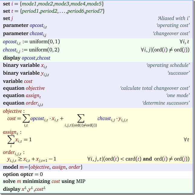
A somewhat strange scheduling model was presented to me. We operate a machine in one of several operating modes \(i\). We have time periods \(t\) and the operating cost \(c^{op}_{i,t}\) changes over time. Obviously, the best schedule would be to pick in each period \(t\) the cheapest operating mode. Now we add a changeover cost: when we change from mode \(i\) to mode \(j\) we pay some cost \(c^{ch}_{i,j}\). This would require a real optimization model to find the optimal operating sequence.

Here is a simple model to handle this:

image

We have used some random data here, which looks like:

----     12 PARAMETER opcost  operating cost

          period1     period2     period3     period4     period5     period6     period7

mode1       0.172       0.843       0.550       0.301       0.292       0.224       0.350
mode2       0.856       0.067       0.500       0.998       0.579       0.991       0.762
mode3       0.131       0.640       0.160       0.250       0.669       0.435       0.360
mode4       0.351       0.131       0.150       0.589       0.831       0.231       0.666
mode5       0.776       0.304       0.110       0.502       0.160       0.872       0.265


----     12 PARAMETER chcost  changeover cost

            mode1       mode2       mode3       mode4       mode5

mode1                   0.572       1.188       1.445       1.256
mode2       0.928                   0.827       0.235       0.628
mode3       0.093       0.677                   0.364       1.291
mode4       1.121       1.540       0.596                   1.322
mode5       1.512       1.255       0.568       0.173

The solution looks like:

----     34 VARIABLE x.L  operating schedule

          period1     period2     period3     period4     period5     period6     period7

mode1                                                           1           1           1
mode3           1           1           1           1


----     34 VARIABLE y.L  successor

                period4

mode3.mode1           1


----     34 VARIABLE cost.L                =        2.139 

We see one changeover between periods 4 and 5. Notice that \(y\) is defined in the model above as:
\[y_{i,j,t} = \begin{cases} 1 \> \text{if $x_{i,t}=1$ and $x_{i,t+1}=1$} \\
                                      0 \> \text{otherwise}\end{cases}\]

This can also be interpreted as a nonlinear constraint \(y_{i,j,t} = x_{i,t}x_{i,t+1}\). In the model we have linearized this. A refinement of the model would have us look at the operating mode just before we start scheduling (i.e. the operating mode in period 0). To handle that easily it is helpful to change the definition of \(y\) to:
\[y_{i,j,t} = \begin{cases} 1 \> \text{if $x_{i,t-1}=1$ and $x_{i,t}=1$} \\
                                      0 \> \text{otherwise}\end{cases}\]

Only equation order needs to change:

image

Note that \(x0\) is an extremely sparse matrix: it has only one element corresponding to the operating mode for the machine just before period 1. (We used here a GAMS feature: addressing lags outside the domain cause the symbol to be dropped; so \(x_{i,t-1}\) for \(t=period1\) will disappear; in that special case the parameter \(x0\) will kick in). The final results with this initial changeover cost is:

----     37 VARIABLE x.L  operating schedule

          period1     period2     period3     period4     period5     period6     period7

mode1                                                           1           1           1
mode3                                               1
mode4           1           1           1


----     37 VARIABLE y.L  successor

                period4     period5

mode3.mode1                       1
mode4.mode3           1


----     37 VARIABLE cost.L                =        2.438

Note that the initial mode in period 0 was 4, and now we keep operating using that mode for a little while.

Wednesday, May 18, 2016

Finding all solutions of a system of linear inequalities III

An easier method to find all corner points for a system of linear inequalities is to encode the basis using binary variables and then use the Cplex solution pool. Here we used a loop where we added binary cuts to prevent an earlier found basis to be revisited again. A complete description of the problem can be found in that post also. With the Cplex solution pool we just use one solve and we don’t have to bother with specifying the cuts. In addition we expect to see much of a performance improvement. So how does performance stack up with the loop?

image

As we can see the performance of the solution pool is superior compared to the loop implementation. Note: it will give the same solution (although in a different order).

Model

The complete model listing is here:

*-----------------------------------
* original model equations
*-----------------------------------

set
  k   
'rows+columns' /1*5,r1*r5/
  j(k)
'columns'      /1*5/
  i(k)
'rows'         /r1*r5/
  bnd 
'bounds'       /lo,up/
;


variables
   x(j) 
'original decision variables'
   r(i) 
'row levels'
;
equations
  e1,e2,e3,e4,e5
;

e1.. r(
'r1') =e= 5*x('1')+3*x('2')+3*x('3')+5*x('4');
e2.. r(
'r2') =e= x('2')+x('3'
);
e3.. r(
'r3') =e= x('1')+x('4'
);
e4.. r(
'r4') =e= 3*x('3')+5*x('4'
);
e5.. r(
'r5') =e= 5*x('1')+3*x('2'
);

table
rowbound(i,bnd)
   
lo up

r1   3  5
r2      1
r3      1
r4   1  3
r5      2
;

r.lo(i) = rowbound(i,
'lo');
r.up(i) = rowbound(i,
'up'
);
x.lo(j) = 0;
x.up(j) = 1;

*-----------------------------------

* basis encoding using
* binary variables
*-----------------------------------

scalar m 'number of LP rows';
m =
card
(i);

set b 'basis status'

     
/NBLO  'nonbasic at lower bound'
      
NBUP  'nonbasic at upper bound'
      
B     'basic'/
;
binary variables
   bs(k,b)
'basis status of each row and column'
;

equations
  onebs(k)  
'only basis status is current'
  countb    
'number of basics = m'
  vlower(j) 
'variable is nb at lower'
  rlower(i) 
'row is nb at lower'
  vupper(j) 
'variable is nb at upper'
  rupper(i) 
'row is nb at upper'
;

onebs(k)..  
sum(b, bs(k,b)) =e= 1;
countb..    
sum(k, bs(k,'B'
)) =e= m;
vlower(j)..  x(j) =l= x.lo(j) + (x.up(j)-x.lo(j))*(1-bs(j,
'NBLO'
));
rlower(i)..  r(i) =l= r.lo(i) + (r.up(i)-r.lo(i))*(1-bs(i,
'NBLO'
));
vupper(j)..  x(j) =g= x.up(j) - (x.up(j)-x.lo(j))*(1-bs(j,
'NBUP'
));
rupper(i)..  r(i) =g= r.up(i) - (r.up(i)-r.lo(i))*(1-bs(i,
'NBUP'
));

*-----------------------------------

* dummy objective
*-----------------------------------

equation edummy;
variable
dummy;
edummy.. dummy =e= 0;

*-----------------------------------

* model statement
*-----------------------------------

model Model1 /all/;
Model1.solvelink=%Solvelink.LoadLibrary%;
Model1.solprint=%Solprint.Quiet%;

option
optcr=0;
option
mip=cplex;

*-----------------------------------

* solution pool solve
*-----------------------------------


$onecho > cplex.opt
SolnPoolAGap = 0.0
SolnPoolIntensity = 4
PopulateLim = 10000
SolnPoolPop = 2
solnpoolmerge solutions.gdx
$offecho

model1.optfile=1;
Solve Model1 using mip minimizing dummy;


*-----------------------------------

* read solution data
*-----------------------------------

sets
  p
'solution points' /soln_model1_p1*soln_model1_p1000/
  c(p)
;
parameters
  v(p,k)
'collect values'
  bas(p,k,b)
'collect basis status'
;
execute_load "solutions.gdx",v=x,bas=bs,c=index;


*-----------------------------------

* remove duplicate values
*-----------------------------------

parameters
  w(k,p)
'unique values'
  found
/0/
;

set u(p) 'subset of index';
u(p) =
no
;

loop
(c,
 
if(card
(u)=0,
    u(c) =
yes
;
    w(k,c) = v(c,k);
 
else

     found = 0;
    
loop(u$(not found),
       found$(
sum
(k,abs(w(k,u)-v(c,k)))<1.0e-5) = 1;
     );
    
if(not
found,
        u(c) =
yes
;
        w(k,c) = v(c,k);
     );
  );
);

display
w;

Finding all solutions of a system of linear inequalities II

In this post (a followup to this one), I want to find all corner points related to these inequalities:
\[\boxed{\begin{align} &3 \le 5x_1+3x_2+3x_3+5x_4 \le 5 \\ &0 \le x_2+x_3 \le 1 \\ &0 \le x_1+x_4 \le 1 \\ &1 \le 3x_3+5x_4 \le 3 \\ &0 \le 5x_1+3x_2 \le 2 \\ &0 \le x_1,x_2,x_3,x_4 \le 1 \end{align}}\]
The approach I follow is based on this post. That is, we use binary variables to explicitly encode the LP  basis, and then solve a series of MIP models where we add cuts to the model to exclude the currently found basis. There are two main differences with the model shown  in the original post:

  • The current problem has no objective. This is not a major hurdle: we can add a dummy objective. The algorithm becomes actually slightly easier as we don't have to check if the objective starts to deteriorate.
  • The current problem has bounded variables. In the original problem we assumed we have positive variables without an upper bound. That meant we could use a single binary variable to encode the basis status: a variable is basic or non-basic. In the current case we could do the same thing and implement the bounds as explicit constraints. However, instead I choose for a slightly more sophisticated approach: we allow the basis status to assume three different values: basic, non-basic at lower bound and non-basic at upper bound. This is exactly how Simplex based linear programming solvers deal with bounded variables.

Positive variables/slacks

Let’s recapitulate what we did in the case of positive variables. When we have positive variables (or slacks) \(x_k\ge 0\), we can use the following basis encoding:
\[\beta_k = \begin{cases} 1 \> \text{if \(x_k\) is basic}\\
                                   0 \> \text{if \(x_k\) is non-basic} \end{cases}\]
If a variable is non-basic it should be equal to zero. This is implemented as
\[0 \le x_k \le M \beta_k\]
In addition we know that we have \(m\) (number of LP rows) basics:
\[\sum_k \beta_k = m\]

Bounded variables/slacks

To handle bounded variables (and slacks): \(\ell_k \le x_k \le u_k\), we introduce an index \(b=\{\text{B,NBLO,NBUP}\}\), where B means basic (variable is between its bounds), NBLO means nonbasic at lower bound (i.e. \(x_k = \ell_k\)) and NBUP means nonbasic upper (\(x_k=u_k\)). Now we can write:
\[\beta_{k,b} = \begin{cases} 1 \> \text{if \(x_k\) has basis status \(b\)}\\
                                                 0 \> \text{otherwise}\end{cases}\]
Of course each variable can assume only one (and exactly one) basis status:
\[\sum_b \beta_{k,b} = 1 \> \forall k\]
If a variable is non-basic, it should be at bound:
\[\begin{align} & \ell_k \le x_k \le \ell_k + (u_k-\ell_k)(1-\beta_{k,\text{NBLO}})\\
                     & u_k \ge x_k \ge u_k - (u_k-\ell_k)(1-\beta_{k,\text{NBUP}}) \end{align}\]
Again, we have \(m\) basics:
\[\sum_k \beta_{k,\text{B}} = m\]

Solution

After running the model we have a large number of feasible bases, 767 to be precise. Some partial results are listed below:

image

The top part are the values of the columns and rows. The bottom part shows the basis status. We see we get some duplicate values (they have a different basis, but the same values; this is called degeneracy in linear programming).

We can easily add some code to the model to find the unique values and filter out the duplicates:

image

There are only 20 unique corner point solutions.

We had to run 768 models for that (the last model was infeasible so we stopped), and every model became larger by one constraint. That also means models are becoming more expensive to solve. This is illustrated in this graph: both the number of Simplex Iterations needed to solve each model (orange line) and the solution times (blue line) show an increase over time.

image

Model

Below the complete model is listed:

*-----------------------------------
* original model equations
*-----------------------------------

set
  k   
'rows+columns' /1*5,r1*r5/
  j(k)
'columns'      /1*5/
  i(k)
'rows'         /r1*r5/
  bnd 
'bounds'       /lo,up/
;


variables
   x(j) 
'original decision variables'
   r(i) 
'row levels'
;
equations
  e1,e2,e3,e4,e5
;

e1.. r(
'r1') =e= 5*x('1')+3*x('2')+3*x('3')+5*x('4');
e2.. r(
'r2') =e= x('2')+x('3'
);
e3.. r(
'r3') =e= x('1')+x('4'
);
e4.. r(
'r4') =e= 3*x('3')+5*x('4'
);
e5.. r(
'r5') =e= 5*x('1')+3*x('2'
);

table
rowbound(i,bnd)
   
lo up

r1   3  5
r2      1
r3      1
r4   1  3
r5      2
;

r.lo(i) = rowbound(i,
'lo');
r.up(i) = rowbound(i,
'up'
);
x.lo(j) = 0;
x.up(j) = 1;

*-----------------------------------

* basis encoding using
* binary variables
*-----------------------------------

scalar m 'number of LP rows';
m =
card
(i);

set b 'basis status'

     
/NBLO  'nonbasic at lower bound'
      
NBUP  'nonbasic at upper bound'
      
B     'basic'/
;
binary variables
   bs(k,b)
'basis status of each row and column'
;

equations
  onebs(k)  
'only basis status is current'
  countb    
'number of basics = m'
  vlower(j) 
'variable is nb at lower'
  rlower(i) 
'row is nb at lower'
  vupper(j) 
'variable is nb at upper'
  rupper(i) 
'row is nb at upper'
;

onebs(k)..  
sum(b, bs(k,b)) =e= 1;
countb..    
sum(k, bs(k,'B'
)) =e= m;
vlower(j)..  x(j) =l= x.lo(j) + (x.up(j)-x.lo(j))*(1-bs(j,
'NBLO'
));
rlower(i)..  r(i) =l= r.lo(i) + (r.up(i)-r.lo(i))*(1-bs(i,
'NBLO'
));
vupper(j)..  x(j) =g= x.up(j) - (x.up(j)-x.lo(j))*(1-bs(j,
'NBUP'
));
rupper(i)..  r(i) =g= r.up(i) - (r.up(i)-r.lo(i))*(1-bs(i,
'NBUP'
));


*-----------------------------------

* cuts to prevent revisiting
* same basis
*-----------------------------------

set
   iter
'iterations' /iter1*iter1000/
   c(iter)
'used cuts'
;
parameter cc(iter,k,b) 'cut-coefficients';
scalar
nn;
nn =
card
(k);

equation
cuts(iter);
cuts(c)..
sum
((k,b),cc(c,k,b)*bs(k,b)) =l= nn-1;

c(iter) =
no
;
cc(c,k,b) = 0;

*-----------------------------------

* dummy objective
*-----------------------------------

equation edummy;
variable
dummy;
edummy.. dummy =e= 0;

*-----------------------------------

* model statement
*-----------------------------------

model Model1 /all/;
Model1.solvelink=%Solvelink.LoadLibrary%;
Model1.solprint=%Solprint.Quiet%;

option
optcr=0;
option
mip=cplex;

*-----------------------------------

* solve loop
*-----------------------------------

parameters
  v(k,iter)
'collect values'
  bas(k,b,iter)
'collect basis status'
;

scalar continue /1/;
loop
(iter$continue,
  
Solve
Model1 using mip minimizing dummy;
   continue$(Model1.modelstat<>%ModelStat.Optimal%) = 0;
  
if
(continue,
      cc(iter,k,b) = round(bs.l(k,b));
      c(iter) =
yes
;
      v(j,iter) = x.l(j);
      v(i,iter) = r.l(i);
      bas(k,b,iter) = bs.l(k,b);
   );
);

display
v, bas;

*-----------------------------------

* remove duplicate values
*-----------------------------------

parameters
  w(k,iter)
'unique values'
  found
/0/
;

set u(iter) 'subset of c';
u(iter) =
no
;

loop
(c,
 
if(card
(u)=0,
    u(c) =
yes
;
    w(k,c) = v(k,c);
 
else

     found = 0;
    
loop(u$(not found),
       found$(
sum
(k,abs(w(k,u)-v(k,c)))<1.0e-5) = 1;
     );
    
if(not
found,
        u(c) =
yes
;
        w(k,c) = v(k,c);
     );
  );
);

display
w;