Reliability of NLP solvers

NLP solvers can fail for a number of reasons. One way to increase the reliability of a production run is to use a back-up solver in case the main solver fails. In GAMS primal and dual information is passed between SOLVE statements even if different solvers are used. This is actually very useful in a case I just observed.

Solver	Status
mosek	Near Optimal
ipopt	Solved to Acceptable Level
mosek + ipopt	Optimal Solution Found

Here both Mosek and IPOPT are getting into trouble and are not able to give us an optimal solution (in this case it was close, but I have seen cases where “near optimal” could be interpreted as “far away from optimal”). But the sequence: first Mosek, then IPOPT actually solves the problem to optimality.

We programmed this essentially as:

option nlp=mosek;
solve allocationmodel minimizing entropy using nlp;
if (allocationmodel.modelstat > 2,       { not optimal }
    option nlp=ipopt;
    solve allocationmodel minimizing entropy using nlp;
);

k-means clustering heuristic in GAMS and the XOR operator

In http://yetanothermathprogrammingconsultant.blogspot.com/2015/03/k-means-clustering-formulated-as-miqcp.html we were quite underwhelmed by the performance of MIQCPs (Mixed Integer Quadratically Constrained Problems).

A standard heuristic is easily formulated in GAMS:

$ontext   K-means clustering heuristic $offtext option seed=101; sets    k  'clusters' /k1*k4/    i  'data points' /i1*i100/    ik(i,k) 'assignment of points to clusters'    xy 'coordinates of points' /x,y/ ; parameter    m(k,xy) 'random clusters to generate data points'    p(i,*)  'data points'    numk    'number of clusters'    cluster(i)    'cluster number' ; numk = card(k); alias(ii,i); *------------------------------------------------ * generate random data * points are around some clusters *------------------------------------------------ m(k,xy) = uniform(0,4); cluster(i) = uniformint(1,numk); ik(i,k) = cluster(i)=ord(k); p(i,xy) = sum(ik(i,k),m(k,xy)) + uniform(0,1); display m,p; sets   ik(i,k) 'assignment of points to clusters'   ik_prev(i,k) 'previous assignment of points to clusters'   ik_diff   trial   'number of trials' /trial1*trial15/   iter    'max number of iterations' /iter1*iter20/ ; parameters   n(k)       'number of points assigned to cluster'   c(k,xy)    'centroids'   notconverged  '0=converged,else not converged'   d(i,k)     'squared distance'   dclose(i)  'distance closest cluster'   trace(trial,iter) 'reporting' ; loop(trial, *------------------------------------------------ * Step 1 * Random assignment *------------------------------------------------       cluster(i) = uniformint(1,numk);       ik(i,k) = cluster(i)=ord(k);       notConverged = 1;       loop(iter$notConverged, *------------------------------------------------ * Step 2 * Calculate centroids *------------------------------------------------           n(k) = sum(ik(i,k), 1);           c(k,xy)$n(k) = sum(ik(i,k), p(i,xy))/n(k); *------------------------------------------------ * Step 3 * Re-assign points *------------------------------------------------           ik_prev(i,k) = ik(i,k);           d(i,k) = sum(xy, sqr(p(i,xy)-c(k,xy)));           dclose(i) = smin(k, d(i,k));           ik(i,k) = yes$(dclose(i) = d(i,k)); *------------------------------------------------ * Step 4 * Check convergence *------------------------------------------------           ik_diff(i,k) = ik(i,k) xor ik_prev(i,k);           notConverged = card(ik_diff);           trace(trial,iter) = sum(ik(i,k),d(i,k));       ); ); display trace;

The results show it is important to use different starting configurations (i.e. multiple trials):

----    100 PARAMETER trace  reporting               iter1       iter2       iter3       iter4       iter5       iter6 trial1      366.178      28.135      14.566 trial2      271.458      26.741      14.566 trial3      316.975      23.912      14.566 trial4      299.522      24.511      14.566 trial5      346.148      77.747      14.566 trial6      313.978      64.730      14.865      14.566 trial7      310.735      27.412      14.566 trial8      330.829     213.308     184.504     102.191      76.611      74.210 trial9      356.897      90.286      16.112      14.566 trial10     345.086      82.716      76.154      76.146 trial11     354.545     169.648      75.626      74.350      71.929      67.385 trial12     310.257      52.175      18.800      14.566 trial13     289.293      23.505      14.566 trial14     337.024      20.783      14.566 trial15     336.969      28.747      14.566       +       iter7       iter8       iter9      iter10 trial8       67.933      42.621      14.881      14.566 trial11      59.815      59.591

The consensus is that 14.566 is the optimal sum of the squared distances. Note that this was an extremely easy problem:

Notes:

1. We use an xor operator to find the difference between if the sets ik_prev and ik. If there is no difference card(ik_diff)=0 and thus notConverged=0. See below for a small example illustrating the xor.
2. The assignment
   ik(i,k) = yes$(dclose(i) = d(i,k));
   is incorrect if point i is exactly between two clusters. In that case we assign the point to two clusters. We can fix this by a more complicated loop:
   ik(i,k) = no;
   loop((i,k)$(dclose(i) = d(i,k)),
     ik(i,k)$(sum(ik(i,kk),1)=0) = yes;
   );
   
   
3. The construct
   cluster(i) = uniformint(1,numk); ik(i,k) = cluster(i)=ord(k);
   cannot be simplified to 
   ik(i,k) = uniformint(1,numk)=ord(k);. 
   The latter version is incorrect.
4. The assignment
   c(k,xy)$n(k) = sum(ik(i,k), p(i,xy))/n(k); 
   will keep a cluster with zero points at its current location.

The XOR operator

This fragment illustrates a few different ways to calculate the difference between two sets:

set    i /a*z/    j(i) /a,b/    k(i) /  b,c/    diff(i) 'difference between sets: card(diff)=0 if equal' ; diff(i) = (j(i)-k(i)) + (k(i)-j(i)); display diff; diff(i) = j(i) xor k(i); display diff; diff(i) = 1$j(i) <> 1$k(i); display diff;

----      9 SET diff  difference between sets: card(diff)=0 if equal a,    c ----     12 SET diff  difference between sets: card(diff)=0 if equal a,    c ----     15 SET diff  difference between sets: card(diff)=0 if equal a,    c

My preferred syntax diff(i)=j(i)<>k(i) is not allowed. In my opinion, notation should really try to help readability, and not show off mathematical prowess.

More oligopolistic behavior

Even very simple models require attention to detail. In [link] we described simple model from the literature. A related model with a coupling constraint that limits pollution emissions is described in:

1. Jacek Krawczyk and James Zuccollo, NIRA-3: An improved MATLAB package for finding Nash equilibria in infinite games, Victoria University of Wellington, December 2006
2. Lars Mathiesen, Regulation of pollution in a Cournot equilibrium, The Norwegian School of Economics and Business Administration, Bergen, June 2008.

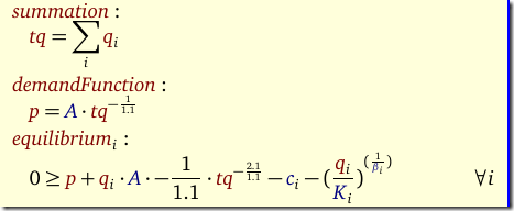
The Nash-Cournot model without pollution controls is simply:

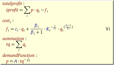
Adding the pollution controls using taxes (or tradable quotas) is not that difficult:

Still for this simple model I get different results for the base case (no pollution controls). My results are:

----    135 PARAMETER results                       output      profit    emission       price no control  .j1      55.351      61.274 no control  .j2      14.914      13.345 no control  .j3      53.684      57.639 no control  .k1                             419.978 no control  .k2                             301.125 no control  .-                                            1.761 with control.j1      21.145       8.942 with control.j2      16.028      15.414 with control.j3       2.726       0.149 with control.k1                             100.000 with control.k2                              81.164 with control.-                                            2.601

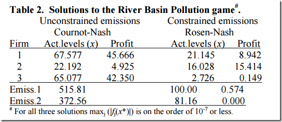
The paper [1] has the following results:

The second part corresponds to my solutions, but the first part shows differences. As the problem with controls is an extension of the problem without controls, there is actually a reasonable chance my solution is correct. 

MIP Links

• Ed Klotz (Cplex): Identification, Assessment and Correction of Ill-Conditioning and Numerical Instability in Linear and Integer Programs [slides and recording].
• Performance Variability
• Performance Variability Defined [link]
• Performance Variability: Good Readings [link]
• Performance Variability: Consequences [link]
• Cplex Performance Variability [link]

K-means clustering formulated as MIQCP optimization problem

It is instructive to formulate the k-means clustering problem as a Mixed-Integer Quadratically Constrained Problem (MIQCP) in GAMS. It looks trivial at first sight but in fact requires a little bit of attention.

We start with a small data set. E.g. 3 clusters and 50 data points in two dimensions (x and y). I.e. our sets look like:

We generate some random clusters as follows:

Should be an easy problem:

The clustering model could look like:

We solver here for two things simultaneously:

1. The location of the clusters (continuous variables c)
2. The assignment of points to clusters (binary variables x)

The equation distances computes all (squared) distances between the points and the clusters. We multiply by x so that we only sum these distances when a point is assigned to a cluster (in that case x=1). Finally we make sure each point is assigned to exactly one cluster.

Unfortunately this model is non-convex, so we can solve this only with global solvers such as Baron or GloMiQo.

Convexification

We can make the model convex as follows:

We use a big-M construct where the upper bound of d forms a reasonable tight value for M. Here we have that d(i,k)=0 if point i is not assigned to cluster k (note that d≥0). The objective has become linear in this case.

Now we can solve the problem with commercial solvers like Cplex and Gurobi. The results (with the location of the clusters from variable c) are:

Performance

For larger data sets it turns out the performance is not very good. E.g. with 100 points and 4 clusters we have 400 binary variables and it takes hours or days to prove optimality. Both Cplex and Gurobi are not able to prove optimality even when we load an optimal solution using MIPSTART. Xpress has even more troubles, and returns bad solutions. We see more often that MIQP/MIQCP solvers are not as robust and fast as (linear) MIP solvers. It is too bad the MIQCP solvers are doing so poorly on this problem.

Using a solver would have opened up possibly interesting extensions like additional constraints on the clustering, such as “at least n points in each cluster”.

Bug in Gurobi

We were able to confuse Gurobi by writing the model as:

It now accepts the model (although it is non-convex) and produces a bogus solution: all points are assigned to cluster 1. Gurobi should have refused to solve the problem (with some message about Q matrix not PSD).

Oligopolistic producer behavior or why airline tickets are not cheaper

Small example from the literature:
 
Note: John Nash just won the Abel prize (http://www.nature.com/news/beautiful-mind-john-nash-adds-abel-prize-to-his-nobel-1.17179).

We implement different behaviors with a GAMS model:

Behavior	Equations
Oligopolistic (MCP) Nash-Cournot Equilibrium
Monopolistic (NLP) Think of this as firms are merged.
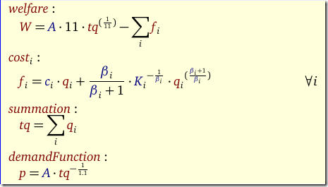
Competitive (NLP) Technique: Optimize Social Welfare Objective. Check solution by: Price= Marginal Cost.

Here q(i) is quantity supplied by firm i. We see most profit is to be made by merging firms and reducing capacity, just as happened in the US airline industry (Europe is a very different story). See also: https://www.nytimes.com/2015/03/24/business/dealbook/as-oil-prices-fall-air-fares-still-stay-high.html.
Another small example from energy markets: https://yetanothermathprogrammingconsultant.blogspot.com/2013/07/microeconomic-principles.html

Sparse sum: set cover problem in GAMS

In a set cover problem (http://en.wikipedia.org/wiki/Set_cover_problem)  we can organize the sets in two different ways:

1. Use a (sparse) two dimensional set. The cover equation will contain a construct like: sum[c(s,i), x(s)].
2. Use a (sparse) zero-one parameter. In this case the cover equation can have something like: sum[s, c(s,i)*x(s)].

The question came up. What is better? I like the set construct a bit better but that is purely based on aesthetics. The performance is exactly the same.

Data structure: set	Data structure: 0/1 parameter

The sets are randomly generated. We solve here just as an LP as we are only interested in the performance of GAMS generating the problem.

gdx2sqlite –fast option

The –fast option in the tool gdx2sqlite is sometimes really helpful. This is especially the case if there are many tables:

The column avg table size indicates the average number of rows in a table. It looks like if this number is small the effect of –fast is most pronounced.

The –fast option will issue PRAGMA synchronous = OFF and PRAGMA journal_mode = MEMORY to SQLite.

---

Here is a nice presentation on SQLite:

Interesting tidbit: statistics on SQLite: 2e9 running instances, 5e5 applications (May 2014).