GDX2SQLite –small option

In the tool GDX2SQLITE we export a GAMS GDX file to a SQLite database file.

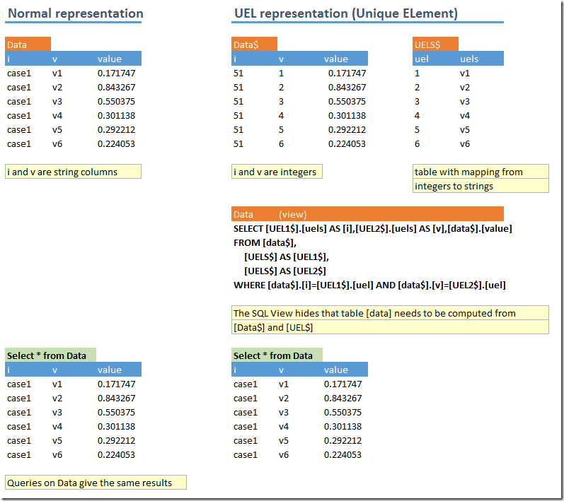
The –small option mimics how GAMS stores data internally. All strings (called UELs or Unique Elements) are stored in a pool and all sets, parameters, variables and equations use index numbers for that pool.

To find out how such a pool looks like, you can do

alias (*,pool);
display pool;

The same storage mechanism is used in GDX files: the strings are stored separately.

When we convert a GDX file to a SQLite database there is an option to use the same storage structure. With SQL we can hide the details behind a VIEW: a “virtual” table that is computed on the fly from an underlying SQL SELECT statement.

Here is the mechanism:

In the picture above, only the first 6 rows of each table are shown. In reality the tables have a significant number of rows.

In practical models and data sets the number of UELS (ie the size of the string pool) is small (often surprisingly small) compared to the total number of rows in the data tables. The advantage of this storage scheme is that the database files are smaller.

Indeed here we have some statistics:

Artificial data often has a larger number of UELs than real world data, as is illustrated here (data.gdx is a synthetic data set while WaterCropData is from a real model).

Notes:

1. A single UEL pool is used for multiple data tables.
2. This somewhat related to older LP solvers which had a super-sparsity storage scheme. Not only were the zero elements not stored but also all values were stored in a pool and the coefficient matrix was pointing into this pool.  I don’t think this scheme is used anymore. Most recent reference I could find is http://www.sciencedirect.com/science/article/pii/0360835290900068. The original reference is:
       KALAN, J., "Aspects of Large-Scale In-Core Linear Programming," ACM Proceedings, 1971
   To be complete: Sparsity indicates we don’t store zero elements. Usually we don’t store zero elements in GDX files (as GAMS does not store and export them). This also means zero elements are not stored in the resulting database file either. E.g. in table Data, only combinations (i,v,value) exist where value ≠ 0.
3. Version 0.5 of GDX2SQLITE adds better column names to the CREATE VIEW statements to make the results more compatible with the default storage scheme.
4. The –small option is clearly beneficial on database size. What are the impacts on performance of creating the database and on querying the database? Creating the database is probably close to linear in the total size, so I expect some savings here. I have no good answer about querying speed. Note: the column uel in table UELS$ is a primary key.

Gurobi vs R: subset selection

The R package leaps (http://cran.r-project.org/web/packages/leaps/leaps.pdf) provided a convenient way to perform feature selection. The methods are based on work by Alan Miller, described in:

Alan Miller, “Subset Selection in Regression”, Chapman and Hall/CRC; 2 edition (April 15, 2002)

In a related paper: Alan Miller, “Subsets of Regression Variables”, J. R. Statist. Soc. A (1984), 147, Part 3, pp. 389-425 (http://citeseerx.ist.psu.edu/viewdoc/download?doi=10.1.1.474.3223&rep=rep1&type=pdf) we even see some comments from Beale.

We should be able to reproduce the “exhaustive” method from the leaps package using an MIQP formulation. Something like:

 

Given a value for n we want to minimize SSQ. The binary variables δ indicate whether a feature j can appear in the model (we exclude the constant term: that one remains in the model). We need to solve this model for n=1,2,3,… To be complete, the other symbols are β: the quantities we want to estimate, data X,y and our big M constant.

I would guess that say Gurobi would do a better job than leaps. As it turns out, it was not easy to beat leaps.

To generate a random model we use a very simplistic scheme. Not sure if this has much in common with real world data sets, but a similar approach was used in Gatu, Kontoghiorghes, “Branch-and-Bound Algorithms for Computing the Best-Subset Regression Models”, Journal of Computational and Graphical Statistics, Volume 15, Number 1, Pages 139–156:

We use N=50 variables in total of which we want to select n=1,2,3,..,10 variables.

GAMS/Gurobi

Here are the results:

----     87 PARAMETER t                    =      112.897  elapsed time of solve loop ----     87 SET selected  selected variables              v5          v6          v8         v11         v13         v19         v31         v32         v35 n1                      YES n2                      YES n3                      YES                                                         YES n4                      YES                                                         YES n5                      YES                                             YES         YES n6                      YES                                             YES         YES                     YES n7                      YES         YES                                 YES         YES                     YES n8                      YES         YES                     YES         YES         YES                     YES n9                      YES         YES                     YES         YES         YES         YES         YES n10         YES         YES         YES         YES         YES         YES         YES                     YES   +         v40         v43 n2          YES n3          YES n4          YES         YES n5          YES         YES n6          YES         YES n7          YES         YES n8          YES         YES n9          YES         YES n10         YES         YES ----     87 PARAMETER rss  residual sum of squares n1  836.651,    n2  836.342,    n3  836.060,    n4  835.869,    n5  835.677,    n6  835.495,    n7  835.330 n8  835.189,    n9  835.075,    n10 834.937 ----     87 PARAMETER solvetime  time for each solve n1   0.080,    n2   0.135,    n3   0.609,    n4   1.951,    n5   3.876,    n6   6.878,    n7  15.971,    n8  21.016 n9  30.122,    n10 27.511

A few notes:

• The model is very sensitive to the size of M. I used M=1000. With M=1e5 we get into trouble. We can see messages like: Warning: max constraint violation (1.2977e-02) exceeds tolerance (possibly due to large matrix coefficient range).This QP formulation is not so easy to solve for Gurobi from a numerical standpoint.
• The RSS is going down when we add variables. As expected.
• Also as expected: the time to solve each sub-problem goes up when we have more variables in the model. “pick n out of N”  constructs often cause performance problems.
  
• I used a small optcr (gap) and 4 threads to make Gurobi fast enough to beat Leaps. (Leaps takes 3 minutes and a loop of 10 solves with Gurobi takes 2 minutes).
• I often like to formulate a separate fit equation as in:
  
  This turns out to be very bad w.r.t. performance. Of course the fit equation forms a completely dense block in the coefficient matrix, something Gurobi was not designed for (it likes sparse structures much better).

R/Leaps

The R code is simply:

d<-dbGetQuery(db,"select * from data") %>% dcast(i ~ v) %>% select(-i)
system.time(r <- regsubsets(y~.,data=d,nvmax=10,really.big=T))

The first line gets the data from the database and applies a pivot operation (from a long, skinny data frame with three columns i,v,value to a wide one with 10 columns v1,v2,v3,…,v10). This trick is useful to remember is this happens a lot when reading data from a database (such data is typically organized in long, skinny tables opposed to a “matrix” organization). The second line calls the regsubsets function from the Leaps package.

The output is:

v1 v10 v11 v12 v13 v14 v15 v16 v17 v18 v19 v2 v20 v21 v22 v23 v24 v25 v26 v27 v28 1 ( 1 ) " " " " " " " " " " " " " " " " " " " " " " " " " " " " " " " " " " " " " " " " " " 2 ( 1 ) " " " " " " " " " " " " " " " " " " " " " " " " " " " " " " " " " " " " " " " " " " 3 ( 1 ) " " " " " " " " " " " " " " " " " " " " " " " " " " " " " " " " " " " " " " " " " " 4 ( 1 ) " " " " " " " " " " " " " " " " " " " " " " " " " " " " " " " " " " " " " " " " " " 5 ( 1 ) " " " " " " " " " " " " " " " " " " " " "*" " " " " " " " " " " " " " " " " " " " " 6 ( 1 ) " " " " " " " " " " " " " " " " " " " " "*" " " " " " " " " " " " " " " " " " " " " 7 ( 1 ) " " " " " " " " " " " " " " " " " " " " "*" " " " " " " " " " " " " " " " " " " " " 8 ( 1 ) " " " " " " " " "*" " " " " " " " " " " "*" " " " " " " " " " " " " " " " " " " " " 9 ( 1 ) " " " " " " " " "*" " " " " " " " " " " "*" " " " " " " " " " " " " " " " " " " " " 10 ( 1 ) " " " " "*" " " "*" " " " " " " " " " " "*" " " " " " " " " " " " " " " " " " " " " v29 v3 v30 v31 v32 v33 v34 v35 v36 v37 v38 v39 v4 v40 v41 v42 v43 v44 v45 v46 v47 1 ( 1 ) " " " " " " " " " " " " " " " " " " " " " " " " " " " " " " " " " " " " " " " " " " 2 ( 1 ) " " " " " " " " " " " " " " " " " " " " " " " " " " "*" " " " " " " " " " " " " " " 3 ( 1 ) " " " " " " "*" " " " " " " " " " " " " " " " " " " "*" " " " " " " " " " " " " " " 4 ( 1 ) " " " " " " "*" " " " " " " " " " " " " " " " " " " "*" " " " " "*" " " " " " " " " 5 ( 1 ) " " " " " " "*" " " " " " " " " " " " " " " " " " " "*" " " " " "*" " " " " " " " " 6 ( 1 ) " " " " " " "*" " " " " " " "*" " " " " " " " " " " "*" " " " " "*" " " " " " " " " 7 ( 1 ) " " " " " " "*" " " " " " " "*" " " " " " " " " " " "*" " " " " "*" " " " " " " " " 8 ( 1 ) " " " " " " "*" " " " " " " "*" " " " " " " " " " " "*" " " " " "*" " " " " " " " " 9 ( 1 ) " " " " " " "*" "*" " " " " "*" " " " " " " " " " " "*" " " " " "*" " " " " " " " " 10 ( 1 ) " " " " " " "*" "*" " " " " "*" " " " " " " " " " " "*" " " " " "*" " " " " " " " " v48 v49 v5 v50 v6 v7 v8 v9 1 ( 1 ) " " " " " " " " "*" " " " " " " 2 ( 1 ) " " " " " " " " "*" " " " " " " 3 ( 1 ) " " " " " " " " "*" " " " " " " 4 ( 1 ) " " " " " " " " "*" " " " " " " 5 ( 1 ) " " " " " " " " "*" " " " " " " 6 ( 1 ) " " " " " " " " "*" " " " " " " 7 ( 1 ) " " " " " " " " "*" " " "*" " " 8 ( 1 ) " " " " " " " " "*" " " "*" " " 9 ( 1 ) " " " " " " " " "*" " " "*" " " 10 ( 1 ) " " " " " " " " "*" " " "*" " " user system elapsed 194.41 0.00 194.44 > summary(r)$rss [1] 836.6514 836.3416 836.1431 835.9519 835.7598 835.5764 835.4079 835.2662 835.1392 835.0116

The sum of squares start out the same but they diverge just a little bit.

The selected variables are much the same as using Gurobi (but there are a few differences here and there). The time is actually close to that of Gurobi. This performance is much better than I expected.   

Logistic Regression (2): least squares is non-convex

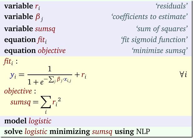
In http://yetanothermathprogrammingconsultant.blogspot.nl/2015/02/logistic-regression.html we implemented a simple maximum likelihood problem which replicates the results from R on a medium size data set (n=400 cases). The question is of course: why can’t we use some least squares objective. The answer is: this problem turns out to be a non-convex problem and thus we may get into trouble.

The can look like:

Of course if you like, we can substitute out the r’s and obtain an unconstrained problem. Note that x and y are data.

Some solvers can solve this, but others have some issues:

Solver	Results
Conopt, Ipopt, Knitro	const -3.94913 gre    0.00211 gpa    0.82281 rank2 -0.69297 rank3 -1.36355 rank4 -1.54693
Minos, Snopt	**** ERRORS/WARNINGS IN EQUATION fit(id1)      1 error(s): exp: FUNC OVERFLOW: x too large (RETURNED 1E299)

Indeed the maximum likelihood version of the model seems easier to solve.

List 64 bit and 32 bit ODBC drivers

It is sometimes a bit confusing to find out which ODBC drivers are installed (especially when we need to know precisely which drivers are 32bit or 64bit). This script when run from a 64 bit GAMS version will list all 32 bit and 64 bit drivers:

$ontext    Run from 64 bit GAMS $offtext $onecho > listodbc.vbs Const HKEY_LOCAL_MACHINE = &H80000002 strComputer = "." Set objRegistry = GetObject("winmgmts:\\" & strComputer & "\root\default:StdRegProv") strKeyPath = "SOFTWARE\ODBC\ODBCINST.INI\ODBC Drivers" objRegistry.EnumValues HKEY_LOCAL_MACHINE, strKeyPath, arrValueNames, arrValueTypes For i = 0 to UBound(arrValueNames)    strValueName = arrValueNames(i)    objRegistry.GetStringValue HKEY_LOCAL_MACHINE,strKeyPath,strValueName,strValue    Wscript.Echo arrValueNames(i) & " -- " & strValue Next $offecho $call echo ===== 64 bit ODBC drivers ======= $call cscript listodbc.vbs //Nologo $call echo ===== 32 bit ODBC drivers ======= $call \windows\syswow64\cscript listodbc.vbs //Nologo

The output looks like:

===== 64 bit ODBC drivers ======= SQL Server -- Installed SQL Server Native Client 11.0 -- Installed ODBC Driver 11 for SQL Server -- Installed ===== 32 bit ODBC drivers ======= Microsoft Access-Treiber (*.mdb) -- Installed Driver do Microsoft Paradox (*.db ) -- Installed Driver do Microsoft Excel(*.xls) -- Installed Microsoft Text Driver (*.txt; *.csv) -- Installed Driver da Microsoft para arquivos texto (*.txt; *.csv) -- Installed Microsoft dBase-Treiber (*.dbf) -- Installed SQL Server -- Installed Microsoft Excel Driver (*.xls) -- Installed Driver do Microsoft dBase (*.dbf) -- Installed Microsoft Paradox-Treiber (*.db ) -- Installed Microsoft ODBC for Oracle -- Installed Microsoft Text-Treiber (*.txt; *.csv) -- Installed Microsoft Excel-Treiber (*.xls) -- Installed Microsoft Access Driver (*.mdb) -- Installed Driver do Microsoft Access (*.mdb) -- Installed Microsoft Paradox Driver (*.db ) -- Installed Microsoft dBase Driver (*.dbf) -- Installed SQL Server Native Client 11.0 -- Installed ODBC Driver 11 for SQL Server -- Installed SQLite3 ODBC Driver -- Installed

See also: http://blogs.technet.com/b/heyscriptingguy/archive/2005/07/07/how-can-i-get-a-list-of-the-odbc-drivers-that-are-installed-on-a-computer.aspx.

Page rank in GAMS

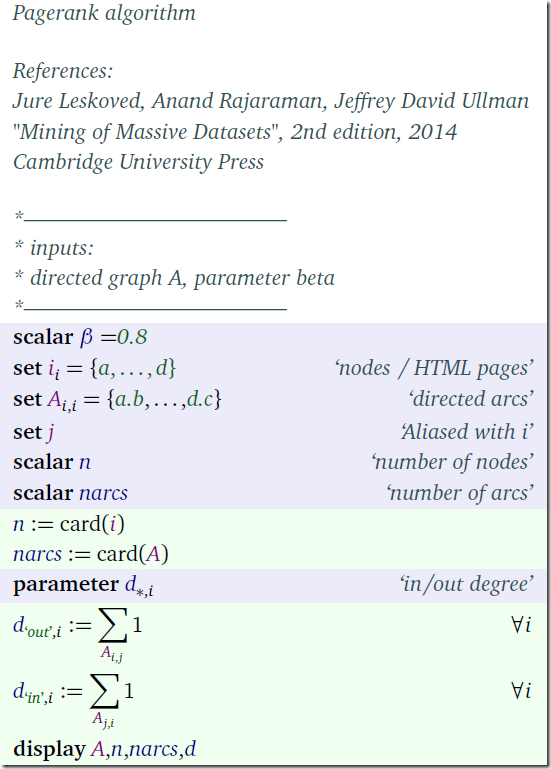
The Google PageRank algorithm is a well known algorithm to calculate web page rankings in a search engine. It is surprisingly simple (for smaller data sets). The basic update equation for the page rank estimate v looks like:

We iterate this thing until the v’s converged. Note that in GAMS this is a parallel assignment so we don’t need to worry about v’s being overwritten during the assignment (otherwise we could have used vprev in the right-hand side expression, see further below). To test this we first load the (sparse) matrix and calculate the degree of each node:

The actual algorithm should perform quite reasonable in GAMS as we can exploit the sparse execution of the matrix-vector multiplication inside the loop. Note that the transition matrix M is transposed wrt A. The loop terminates as soon as the update does not change v anymore.

Indeed I was able to run this model quickly even with the harvard500 data set (http://www.mathworks.com/moler/exm/chapters/pagerank.pdf). For this 500 node web graph the loop takes about 0.5 seconds.

Note: parallel assignment

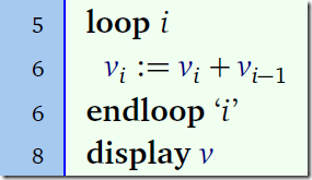
The detail about the parallel assignment can be illustrated with:

In line 4 we set v := [1,2,3,…,10]. After line 5 we have (using parallel assignment): v = [1,2,5,…,19]. If we would have executed:

then we see a result of: v = [1,3,6,…,55].

GAMS vs Matlab

There is no solve in the GAMS code, so Matlab should do very well on this also. In Matlab we can even compare dense vs sparse execution (GAMS always uses sparse storage).

GAMS Sparse M Time: 0.5 s Iterations: 28	loop(iter$(sum(i,abs(v(i)-vprev(i)))>epsilon),    vprev(i)=v(i);    v(i) = beta*sum(j, M(i,j)*v(j)) + (1-beta)/n; );
MATLAB Dense M Time: 0.03 s Iterations: 28	for iter=1:100    vprev=v;    v = beta*M*v + (1-beta)/n;    if (norm(v-vprev,1)<epsilon)        break;    end; end
MATLAB Sparse M Time: 0.01 s Iterations: 28

We can see Matlab is doing much better on the matrix-vector products especially when using a sparse matrix M. The difference between sparse and dense should increase for larger matrices: 500x500 is actually not that big and works quite well with dense linear algebra. The density of the M matrix is 1% in this example and should be smaller for larger matrices. Matlab is very fast as long as we can use the computational kernels efficiently, which is the case here.

Complete code

Here we show the complete model. As it turns out the loop looks quite similar, but some of the initialization code is really different between GAMS and Matlab. Matlab is of course much closer to real mathematical notation than GAMS. I am not sure this always helps in making code more readable. This small example actually shows this succinctly.

GAMS	MATLAB
scalar beta /0.8/; set i 'nodes / HTML pages' /a,b,c,d/; alias(i,j) set a(i,j) 'directed arcs' /   a.(b,c,d)   b.(a,d)   c.c   d.(b,c) /;	beta = 0.8; i = [1,1,1,2,2,3,4,4]; j = [2,3,4,1,4,3,2,3]; A = sparse(i,j,ones(size(i,2),1));
Here we load the data. In GAMS we index over sets consisting of strings. Typically a network graph is implemented as two sets: a one dimensional set with nodes and a two dimensional set with arcs. In Matlab we use matrices where we index over integers 1..n. Here we specify a sparse matrix by providing the row and column numbers; the nonzero values are all one. I prefer the GAMS representation of the graph.
scalars   n   'number of nodes'   narcs  'number of arcs' ; n = card(i); narcs = card(a); parameter d(*,i) 'in/out degree'; d('out',i) = sum(a(i,j),1); d('in',i) = sum(a(j,i),1); display a,n,narcs,d;	n=size(A,1); narcs=nnz(A); d_in = sum(A,1); d_out = sum(A,2);
GAMS needs more lines of code because all identifiers need to be declared before they can be used. This is cumbersome for interactive use but provides extra protection for larger projects. Also GAMS is basically a batch environment (there is no console where we type GAMS commands). GAMS is a very small language. In this model we basically only use the sum operator and the card and abs functions. Matlab has a very rich set of matrix functions (we use here sparse, ones, size, nnz, sum, find, norm). That is of course both a blessing and a curse: we can write things down very compactly but you need to know more stuff before being proficient in Matlab.
set iter /iter1*iter100/; scalars    epsilon 'convergence tolerance' /1e-5/ ; parameter    M(i,j) 'transition matrix j->i'    v(i) 'page rank'    vprev(i) 'page rank from previous iteration' ; * initialization M(i,j)$a(j,i) = 1/d('out',j); display M; v(i) = 1/n; vprev(i) = 0; loop(iter$(sum(i,abs(v(i)-vprev(i)))>epsilon),    vprev(i)=v(i);    v(i) = beta*sum(j, M(i,j)*v(j)) + (1-beta)/n;    display v; ); display v;	epsilon=1.0e-5; k = find(d_out~=0); D = sparse(k,k,1./d_out(k),n,n); M = A' * D; v = ones(n,1)/n; for iter=1:100     vprev=v;     v = beta*M*v + (1-beta)/n;     if (norm(v-vprev,1)<epsilon)          break;     end    end
The construction of the transition matrix M is cleaner in GAMS than in Matlab. It may not be immediately obvious but in the Matlab code the matrix D is a diagonal matrix. Of course we want to store this sparse. The use of a diagonal matrix in Matlab is a well-known trick to keep things vectorized (opposed to using explicit loops). Explicit loops are often bad (i.e. slow) both in GAMS and in Matlab (often beginners tend to overuse loops in both languages). The major iteration loop is programmed in such a way that it always terminates (either by convergence or running out of iterations). This is a useful defensive approach. The test for convergence can be embedded in the loop statement in GAMS (note that this requires vprev to be initialized at this point). In Matlab there is no such trick so we just do the test at the most convenient place. Finally note the difference in the display of the graph A. Arguably the GAMS output is a little bit better to understand. We can improve the Matlab output by saying display(full(A)). Of course we only should do a display of a small graph.
----     38 SET a  directed arcs             a           b           c           d a                     YES         YES         YES b         YES                                 YES c                                 YES d                     YES         YES	>> display(A) A =    (2,1)        1    (1,2)        1    (4,2)        1    (1,3)        1    (3,3)        1    (4,3)        1    (1,4)        1    (2,4)        1

Convergence

The convergence of the term sum(abs(v-vprev)) is interesting. We plot here against the iteration number:

With a logarithmic scale:

Logistic Regression

Logistic regression is a well known technique in statistics. Here we show how we can solve the Maximum Likelihood estimation problem in GAMS. We use the data from http://www.ats.ucla.edu/stat/r/dae/logit.htm.

Of course, here we don’t have a black box logistic regression tool so we need to do a few extra steps. First we need to add an explicit constant term to the data, and expand a categorical variable into a number of dummy variables. The second part is to write down the log likelihood function. The resulting model looks like:

Usually this is written down as an unconstrained optimization problem. In such a formulation we would repeat some linear expressions that I rather substitute out. Largely for aesthetical reasons. This adds a linear constraint block but makes the problem somewhat less nonlinear – depending how you count: the nonlinear code is smaller but the number of nonlinear nonzero elements is larger. For small problems it does not really matter: NLP solvers handle both versions quite well (more details on this below). Yet another way to solve this is to write down the first-order conditions and solve these. I suspect this is how glm inside R works.

Usually for NLP models like this I’d like to specify a starting point for the nonlinear variables. Here it seems that the default initial values bx(i)=0 are just fine.

The GAMS output is:

----    464 VARIABLE beta.L  coefficients to estimate const -3.98998,    gre    0.00226,    gpa    0.80404,    rank2 -0.67544 rank3 -1.34020,    rank4 -1.55146

With R’s glm command we get the same results:

Statistics

Using a little bit of extra code we can calculate some useful statistics. Just as R does. In fact we try to mimic their output. Here is the GAMS code:

We use a small CNS model (square nonlinear system solver) to invert the information matrix. The right-hand side of equation inverter is actually an identity matrix (ones on the diagonal, zero everywhere else). We solve here a linear system of equations with a non-linear solver. That is because GAMS does not have model type to solve a linear system of equations. It could be done with an LP solver and a dummy objective. As the size of the matrix is small, we choose for the shortest GAMS code. The final results when displaying the results parameter look like:

----    487 PARAMETER results           Estimate  Std. Error     z value    Pr(>|z|) const    -3.98998     1.13995    -3.50013     0.00047 gre       0.00226     0.00109     2.06986     0.03847 gpa       0.80404     0.33182     2.42312     0.01539 rank2    -0.67544     0.31649    -2.13417     0.03283 rank3    -1.34020     0.34531    -3.88120     0.00010 rank4    -1.55146     0.41783    -3.71313     0.00020

The estimates are our beta’s. The standard errors are the square root of the diagonal elements of the inverse of the information matrix. The z-values are just the result of dividing the estimate by its standard error. Finally the p-values are found using the standard normal cdf function. This looks just like the R summary output (apart from the stars indicating the significance level):

Coefficients: Estimate Std. Error z value Pr(>|z|) (Intercept) -3.989979 1.139951 -3.500 0.000465 *** gre 0.002264 0.001094 2.070 0.038465 * gpa 0.804038 0.331819 2.423 0.015388 * rank2 -0.675443 0.316490 -2.134 0.032829 * rank3 -1.340204 0.345306 -3.881 0.000104 *** rank4 -1.551464 0.417832 -3.713 0.000205 *** --- Signif. codes: 0 ‘***’ 0.001 ‘**’ 0.01 ‘*’ 0.05 ‘.’ 0.1 ‘ ’ 1

It is actually quite instructive to do this exercise to understand a little bit better what R is reporting when doing a logistic regression. High-performance,  convenient and well-tested black-box routines are great to use. But once in a while it may make sense to go back to basics and work on the problem directly.

Comparison between unconstrained and linearly constrained formulation

I was a little bit wondering about the relative performance of these two different formulations. Here is a summary:

For most solvers it is a wash.