Excel 2010

Reading a bit about Office 2010.

• Excel has now a 64 bit version. The hard limits on rows columns have not been changed, but with 64 bit you can populate them all. Moving to 64 bit has lots of implications w.r.t. OLE, etc. so I would not do this unless really needed. (http://msdn.microsoft.com/en-us/library/ee691831(office.14).aspx, http://www.pcworld.com/article/197415/beware_of_office_2010s_64bit_shortcomings.html)
• Some statistical and other functions have been improved w.r.t accuracy. (http://technet.microsoft.com/en-us/library/cc179167.aspx). May be this solves the problem described here: http://yetanothermathprogrammingconsultant.blogspot.com/2009/05/excel-and-statistics.html.
• Solver has some improvements (including a genetic algorithm based solver) (http://technet.microsoft.com/en-us/library/cc179167.aspx).
• Powerpivot (http://www.powerpivot.com/)
• 64 bit version has some parallel HPC facilities (http://technet.microsoft.com/en-us/library/cc179167.aspx).

GAMS model to stress memory

This model can be used to see if you can allocate say 2 GB of memory.

$ontext    Check if memory can be allocated    erwin@amsterdamoptimization.com $offtext * specify limit in MB * e.g. 2 GB = 2000 scalar maxmem / 2000 /; set i 'keep small to reduce memory here' /i1*i100/; alias (i,i1,i2,i3,i4,i5); parameter p(i,i,i,i,i); loop((i1,i2,i3)$(heapsize<maxmem),    p(i1,i2,i3,i4,i5) = 1; ); scalar numcells "number of cells we could allocate (million)"; numcells = card(p)/1e6; scalar percell "approx bytes per cell"; percell = floor(heapsize/numcells); display numcells,percell;

This is written in response to issue 1 in http://yetanothermathprogrammingconsultant.blogspot.com/2010/05/linux-issues.html.

As an aside it will print the number of bytes per nonzero element in a parameter. As GAMS stores all data sparse, this number is larger than 8 bytes. For 32 bit GAMS systems this number can be 24 bytes per nonzero and for 64 bit systems 32 bytes per nonzero can be expected (pointers need 64 bits instead of 32 bits so memory per cell goes up).

Notes:

• If your machine does not have > 4GB of memory, you can probably solve larger models using 32 bit GAMS on 64 bit Linux
• GAMS reports MB’s as 1000 × 1000 bytes. Other tools may use 2¹⁰=1024 in this calculation.

Linux issues

Linux is often mentioned as a reliable server platform. In the last few days I got two error messages from users that really caused confusion:

The first case is running a large GAMS job, that terminates with:

*** Error: Could not spawn gamscmex, rc = 1
gams: Could not spawn gamscmex, rc = 1

After asking more questions and running a small GAMS test model that allocates > 2 GB, we could conclude the server is running out of memory and the OS starts to kill some large processes, gamscmex being one of them. The message is of course not very informative. May be perror/strerror would have given a better message.

Apparently Linux needs to get rid of processes now and then. Not thinking this through I would think it would be better if it would not kill a process but rather does not parcel out new memory to user processes (i.e. let the malloc fail as soon as memory is exhausted, instead of giving out more memory than you have). Well, anyway. It seems that candidates are processes that started recently but with lots of memory requirements (http://linux-mm.org/OOM_Killer). Here is more info about why: http://lwn.net/Articles/317814/; Linux seems to allow over-committing memory by default. One of the reasons is the fork system call: this can often cause larger memory requests than actually needed – think about a large process spawning a small process, hence the invention of allowing this over-commitment. (Here is a funny analog: http://lwn.net/Articles/104185/).

Here is another one. When gdxls encounters an error (in this case the properties file was not available or incorrectly named) it will print a Java stack trace. Well, in some cases a user saw:

GDXLS V 0.3, Amsterdam Optimization (c) 2008-2010

spcolprop.txt (No such file or directory)

Exception in thread "main" java.lang.NullPointerException
*** Got java.lang.NullPointerException while trying to print stack trace.

I suspect somehow a problem in the Java runtime here.

Good error messages are very important and can really reduce support costs. Error messages are issued when the user is possibly doing something wrong. Confusing an already confused user by a confusing error message only increases the confusion. The messages mentioned in this post are a good example of the indirect cost of lousy messages: users email the problem, even I don’t understand what is happening, and a lot of back-and-forth is needed before we can (approximately) conclude what is going on.

Nordhaus models in Excel

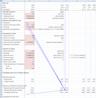
The older DICE (Dynamic Integrated Model of Climate and the Economy) models were available in GAMS and Excel (http://nordhaus.econ.yale.edu/DICE2007.htm). The latest RICE model is only available in Excel (http://nordhaus.econ.yale.edu/RICEmodels.htm). For a project I was studying how the Sea-Level Rise (SLR) functionality was incorporated in the model. I noticed a few places where the Excel formula’s have somewhat surprising forms. They may be bugs or it may be harmless.

The first case is where a series of formula’s calculating the Cumulative Melt for Glaciers and Small Ice Caps. This is row 42 in sheet SLR of http://nordhaus.econ.yale.edu/documents/RICE_042510.xlsm. The formula’s use cell B44 which is empty.

The second case is where a series of formula’s for different years suddenly use a different constant. This is in row 55 in the same sheet SLR (melt rate for Antarctic Ice Sheet). For up to 2115 the formula refers to B25 (Intercept), and after that it uses B24 (Initial Melt Rate).

I am not sure these are bugs, but this certainly looks as a mistake.

Of course I would prefer the models to be available in GAMS. That would probably have prevented errors like this. Without doubt, maintaining two different versions is difficult, and they can easily get out-of-sync. In a different paper (http://www.seas.harvard.edu/climate/pdf/Fuessel.pdf) it is argued that the GAMS and Excel versions of DICE contain different formulations, illustrating my point.

Of course we must applaud Nordhaus for making this work publicly available. That invites criticism. However if people (like me) take the effort to study and comment on the models, that is also a sign that these models actually do matter.

I have notified the author of these (possible) bugs.

Update: The first issue is a bug, but with limited effect in the long run. The second issue is actually as intended: a change in calibration to make things more in line with other results.

Generating random variables having a GAMMA distribution

In GAMS models I often use the following simple algorithm to generate random variable:

1. Generate u = Uniform(0,1)
2. Solve F(x) = u

E.g. for the GAMMA distribution:

$ontext    generate Gamma variates    erwin@amsterdamoptimization.com $offtext set i /i1*i25/; * draw from gamma distribution with mean = 100 scalars   c0  'aka k'      /1.5/   b0  'aka theta'   m0  'mean'       /100/ ; * m=bc b0 = m0/c0; display b0,c0,m0; abort$(abs(m0 - b0*c0) > 0.001) "calculation of c0 was not correct"; parameter u(i); u(i) = uniform(0.001,0.999); display u; variable x(i); equation f(i); f(i).. gammareg(x(i)/b0,c0) =e= u(i); model m /f/; x.lo(i) = 0; x.l(i) = m0; option cns=conopt; solve m using cns; scalar avg; avg = sum(i,x.l(i))/card(i); display avg;

Using a numerical procedure is always dangerous, as we see here:

C O N O P T 3   version 3.14T    Copyright (C)   ARKI Consulting and Development A/S                    Bagsvaerdvej 246 A                    DK-2880 Bagsvaerd, Denmark Using default options. Reading Data   Iter Phase Ninf   Infeasibility   RGmax    NSB   Step InItr MX OK      0   0        6.8475654921E+00 (Input point) ** An equation in the pre-triangular part of the model cannot    be solved because the pivot is too small.    Adding a bound or initial value may help.

The CDF of the Gamma distribution looks quite innocent:

Two simple ways of working around this. First PATH seems to handle this a little bit better (and CONOPT agrees with the solution). This can be done with:

option cns=path; solve m using cns; option cns=conopt; solve m using cns;

Indeed CONOPT new says:

C O N O P T 3   version 3.14T    Copyright (C)   ARKI Consulting and Development A/S                    Bagsvaerdvej 246 A                    DK-2880 Bagsvaerd, Denmark Using default options. Reading Data   Iter Phase Ninf   Infeasibility   RGmax    NSB   Step InItr MX OK      0   0        7.9597856362E-09 (Input point)                                Pre-triangular equations:       25                                Post-triangular equations:       0      1   0        0.0000000000E+00 (After pre-processing)      2   0        0.0000000000E+00 (After scaling)      2            0.0000000000E+00 ** Feasible solution to a square system.

Another solution would be to use a different starting point. We used the mean which is an obvious starting point, but with

x.l(i) = 1;

instead of

x.l(i) = m0;

CONOPT can also solve the equations directly.

This illustrates that, although we can work around things, it would be better to have a larger number of statistical functions in GAMS, including some inverse CDF’s.

Max likelihood estimation with income classes

Typically income data is presented in income classes:

Income Class	Number of Observations
0-$20000	1036
$20000-$40000	495
$40000-$60000	201
$60000-$80000	102
$80000+	38

In order to find the mean income based on such data we can fit e.g. a Pareto Distribution. One way of doing this is with a max likelihood estimation procedure. From http://www.math.uconn.edu/~valdez/math3632s10/M3632Week10-S2010.pdf we have:

(EQ.1)

This is easy to code in GAMS, using a Pareto distribution:

set j 'bins' /b1*b5/; table bin(j,*)         lo     up   observations b1       0  20000      1036 b2   20000  40000       495 b3   40000  60000       201 b4   60000  80000       102 b5   80000    INF        38 ; parameters n(j),lo(j),up(j); lo(j) = bin(j,'lo'); up(j) = bin(j,'up'); n(j) = bin(j,'observations'); * Pareto distribution * See: Evans, Hastings, Peacock, "Statistical Distributions", 3rd ed, Wiley 2000 * find mean income using MLE variables a,c,L; equation loglik; a.lo=1; c.lo=1; a.l = 100; c.l = 1; loglik.. L =e= sum(j, n(j) * log[ (1-(a/up(j))**c)$(ord(j)<card(j)) + 1$(ord(j)=card(j))                                 - (1-(a/lo(j))**c)$(ord(j)>1) - 0$(ord(j)=1)] ); option optcr=0; model mle /all/; parameter mean; solve mle maximizing L using nlp; mean = c.l*a.l/(c.l-1); display mean;

We use here that F(0) = 0 and F(INF) = 1 for the CDF of the Pareto distribution.

Note this approach can be also used to estimate the number of millionaires (ie income > 1e6) even though this number is hidden in the last income class.

Looking at http://www.jstor.org/stable/1914015 I was a little bit confused by

(EQ.2)

however I think we can arrive at the earlier likelihood function. The factor n! can be dropped as it is constant. Taking logs we see:

(EQ.3)

The last sum can be dropped as it is also constant. (Of course this can also be deducted directly from the product in EQ2).

Sun VirtualBox

For a free alternative to VMWare see http://www.virtualbox.org/. It actually works pretty well. Here I am running Ubuntu Linux on a (cheap) laptop. Make sure to install the Guest Additions so you can resize the window.

GCJ: missing %g, %f in format

During some maintenance on gdxls I encountered a bug in the GNU Java system: http://gcc.gnu.org/ml/java/2010-05/msg00004.html. Looking at the reply, this is already there for a while: http://gcc.gnu.org/bugzilla/show_bug.cgi?id=32809. Often problems in GCC are quickly fixed, but as this demonstrates not always.

Large optimization models in Excel?

I was asked to give my opinion on implementing a fairly large and complex optimization model in Excel. Excel is an extremely popular tool in business environments, and often there are people available with skills and experience that can do amazing things with Excel. Even in some academic circles the notion of doing serious optimization modeling in Excel is put forward: http://papers.ssrn.com/sol3/papers.cfm?abstract_id=1088420.

In my experience it is often a good idea to use Excel where it really excels: data-entry and reporting. Lots of the more complicated data manipulation and the implementation of model equations can often better be delegated to specialized modeling software.

I often use Excel Excel as front-end for optimization models. But I try to move data as quickly to the modeling system where we can do data preparation (and checks) in a more systematic way. Similarly, I try to prepare output data in the modeling system and pass it back as late as possible to Excel for reporting (display and graphing).

Of course where to put the boundary between Excel and the modeling system can depend on different criteria. Sometimes this is dictated by technology (a modeling system that does not allow you to do data manipulation forces you to do more in Excel; but more capable systems don’t have this restriction).

An interesting book about Excel is: Professional Excel Development. It has a somewhat different approach than traditional programming books.