Some TSP MTZ experiments

In [1], a question was posed about a TSP model using the MTZ (Miller-Tucker-Zemlin) subtour elimination constraints. The results with Julia/glpk were disappointing. With \(n=58\) cities, things were taken so long that the solver seemed to hang. Here I want to see how a precise formulation with a good MIP solver can do better. As seeing is believing, let's do some experiments. 

The standard MTZ formulation[1] can be derived easily. We use the binary variables \[\color{darkred}x_{i,j}=\begin{cases}1 & \text{if city $j$ is visited directly after going to city $i$}\\ 0 & \text{otherwise}\end{cases}\]  

The building blocks of this TSP model are

• a set of assignment constraints that implement "each city \(i\) has exactly one follower \(j\) and each city \(j\) has exactly one predecessor \(i\)", This yields \[\begin{align}&\sum_{j|i\ne j} \color{darkred}x_{i,j}=1&&\forall i\\ & \sum_{i|i\ne j} \color{darkred}x_{i,j}=1&&\forall j\end{align}\]
• a set of subtour elimination constraints that impose a sequence of cities to visit. This can be modeled as using extra sequencing variables \(\color{darkred}u_i\in\{0,n-1\}\), and the constraint: \[\color{darkred}x_{i,j}=1\implies \color{darkred}u_j=\color{darkred}u_i+1\>\>\forall i\ne j, j \gt 1\] We can fix in advance \(\color{darkred}u_1 = 0\). We can reformulate this constraint as a big-M constraint: \[\color{darkred}u_j \ge \color{darkred}u_i + 1 - \color{darkblue}n\cdot(1-\color{darkred}x_{i,j})\>\>\forall i\ne j, j \gt 1\]

A complete MTZ model can look like:

TSP/MTZ model

\[\begin{align}\min&\sum_{i,j|i\ne j}\color{darkblue}{\mathit{dist}}_{i,j}\cdot\color{darkred}x_{i,j}\\ & \sum_{j|i\ne j} \color{darkred}x_{i,j}=1 && \forall i \\ & \sum_{i|i\ne j} \color{darkred}x_{i,j}=1&&\forall j\\ & \color{darkred}u_j \ge \color{darkred}u_i + 1 - \color{darkblue}n\cdot(1-\color{darkred}x_{i,j}) && \forall i\ne j, j \gt 1 \\ & \color{darkred}u_1 = 0 \\ & \color{darkred}x_{i,j}\in\{0,1\}\\ & \color{darkred}u_i \in \{0,\dots,\color{darkblue}n-1\}\end{align}\]

We can add: \[\begin{align}&  \color{darkred}u_i \ge 1 &&\forall i\gt 1\\ &\sum_i  \color{darkred}u_i = \frac{\color{darkblue}n(\color{darkblue}n-1)}{2} \end{align}\] These are not in the standard MTZ model, and I left them out.

We can relax the \(\color{darkred}u_i\) variables to be continuous. It is not obvious to me, how this affects the computation time. One could argue that the use of continuous variables lead to fewer discrete variables, and this can mean fewer branches, while integer variables convey more information for the presolvers and possibly better cut generation. This is an obvious question which I hardly see discussed. So let's do some experiments. 

Lifted MTZ Constraints

In [3], a somewhat tighter formulation is proposed, called "lifted MTZ constraints". The subtour elimination constraint is replaced by:\[\color{darkred}u_i-\color{darkred}u_j + (\color{darkblue}n-1)\cdot \color{darkred}x_{i,j} + (\color{darkred}n-3)\cdot \color{darkred}x_{j,i} \le \color{darkblue}n-2\>\>\forall i\ne j, j \gt 1\]

Valid Inequalities

There are some valid inequalities (extra constraints that tighten the formulation) for this model [3]. They look like \[\begin{align}&\color{darkred}u_j\ge 1+(1-\color{darkred}x_{1,j})+(\color{darkblue}n-3)\cdot \color{darkred}x_{j,1} && \forall j \ge 2 \\ &\color{darkred}u_j \le (\color{darkblue}n-1)- (\color{darkblue}n-3)\cdot \color{darkred}x_{1,j} - (1-\color{darkred}x_{j,1}) && \forall j \ge 2\end{align}\]

Results

When I try this on a data set with \(n=58\) cities and random coordinates and Euclidean distances, I get the following results:

----    180 PARAMETER stats  collected statistics

                           obj  iterations       nodes     seconds

MTZ(int u)             569.089 1061905.000   83982.000      27.578
MTZ(relaxed u)         569.089 1153378.000   77797.000      22.953
lifted(int u)          569.089 1623901.000  105898.000      20.094
lifted(relaxed u)      569.089 1287205.000   73390.000      18.610
lift+vi(int u)         569.089  365546.000   27155.000       4.735
lift+vi(relaxed u)     569.089  887140.000   60696.000      14.406

 

 Update.This is just one run. In the comments, Riley notes that it is much better to create a bunch of performance observations (either by different problem sets or by changing the seed -- forcing the solver to use a different path). This is because the variability in the timing of MIP solvers is very large, and can dominate single observations. Here is his picture (using Gurobi):

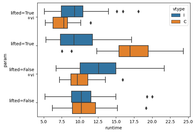Runtimes with 50 replications (using a different seed) using Gurobi

Interestingly to see how integer \(\color{darkred}u_i\) is much better for the lifted case, but not the others. Not sure if I can explain this. May need more replications with different data sets to make sure this difference persists.

These results (with the Cplex MIP solver) indicate that all versions solve within half a minute. The version with the lifted subtour elimination constraint and added valid inequalities using integer \(\color{darkred}u_i\) is surprisingly fast at less than 5 seconds. However, I am not convinced that this particular model is systematically faster than the other ones. I have seen no article that suggests to use integer \(\color{darkred}u_i\). (I have not seen papers even discussing this.) For sure, we can say: there are instances that benefit from using integer variables. It is noted that solvers like Cplex and Gurobi sometimes replace continuous variables with discrete ones. That is not always obvious and requires careful inspection of the log file.

Plot of the results

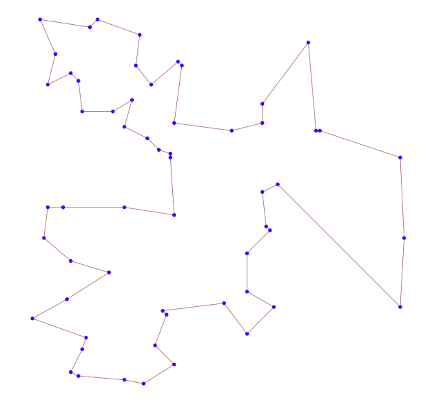
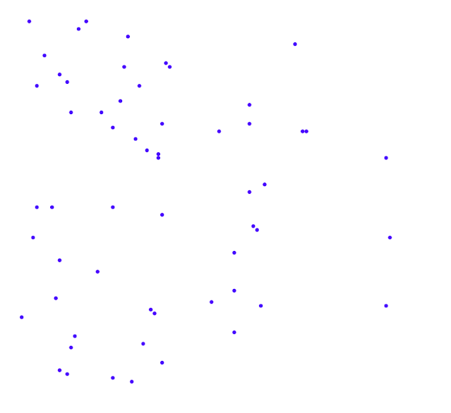
If you look at the plot of the results, the optimal tour seems somewhat obvious. Almost like you could do this by hand. However, if we just view the points, the problem looks much more difficult.

Only the points

It is interesting how I perceive the difficulty of the problem when looking at these two plots. The plot with the optimal tour makes the problem like almost trivial. The plot with just the points makes the problem look quite difficult. This is an example of optical illusion.

Conclusion

The MTZ subtour elimination constraints are known to be slow. A TSP with \(n=58\) points, however, is well within the reach of a good MIP solver. Lifting the MTZ constraints helps a bit, but we are still in the same ballpark. Adding valid inequalities can help further. 

Note that we used an Asymmetric TSP formulation. We don't assume the distances are symmetric, i.e. \(\color{darkblue}{\mathit{dist}}_{i,j}=\color{darkblue}{\mathit{dist}}_{j,i}\). The random dataset, however, has symmetric distances. 

The models don't use callbacks. I stay (somewhat) close to the original MTZ version of the model. I.e., just a straight linear MIP model.

For people using heuristics for this problem: the reported timings are for obtaining proven optimal solutions, not just a good solution.

The GAMS code below also demonstrates a simple way to plot TSP tours. I generate some simple HTML/SVG code for this.

References

1. Julia JuMP slowdown/hang while solving TSP, https://stackoverflow.com/questions/76750379/julia-jump-slowdown-hang-while-solving-tsp
2. Miller, C., A. Tucker, R. Zemlin. 1960, Integer programming formulation of traveling salesman problems. J. ACM 7 326-329
3. Desrochers, M., Laporte, G., Improvements and extensions to the Miller-Tucker-Zemlin subtour elimination constraints, Operations Research Letters, 10 (1991) 27-36.
4. Hanif D. Sherali and Patrick J. Driscoll, On Tightening the Relaxations of Miller-Tucker-Zemlin Formulations for Asymmetric Traveling Salesman Problems, Operations Research, Vol. 50, No. 4 (Jul. - Aug., 2002), pp. 656-669

Appendix 1: GAMS Script

$onText     Simple demo of lifted MTZ     References:       Miller, C., A. Tucker, R. Zemlin. 1960.       Integer programming formulation of traveling       salesman problems. J. ACM 7 326-329           Desrochers, M., Laporte, G.,       Improvements and extensions to the Miller-Tucker-Zemlin       subtour elimination constraints,       Operations Research Letters, 10 (1991) 27-36.   $offText     * use all cores option threads = 0;     *------------------------------------------------------- * data *-------------------------------------------------------   sets    i 'cities' /city1*city58/    xy /x,y/ ; alias(i,j);   scalar n 'number of cities'; n = card(i);   parameter coord(i,xy) 'random coordinates'; coord(i,xy) = uniform(0,100);   parameter dist(i,j) 'distance matrix'; dist(i,j) = sqrt(sum(xy,sqr(coord(i,xy)-coord(j,xy))));   set arcs(i,j) 'travel allowed between cities'; arcs(i,j) = not sameas(i,j);   display n,i,coord,dist,arcs;   *------------------------------------------------------- * reporting macro *-------------------------------------------------------   parameter stats(*,*) 'collected statistics';   $macro statistics(label,model_)  \   stats(label,'obj') = model_.objval;  \   stats(label,'iterations') = model_.iterusd; \   stats(label,'nodes') = model_.nodusd;  \   stats(label,'seconds') = model_.resusd;  \   display stats;     *------------------------------------------------------- * Original MTZ formulation * Integer ordering variables *-------------------------------------------------------   variable totdist 'total distance'; binary variable x(i,j) 'assignment variables: if 1 we travel i->j'; integer variable u(i) 'ordering'; u.up(i) = card(i)-1; * start in city 1 u.fx('city1') = 0;     equations     objective  'sum of distances traveled'     assign1(i) 'assignment constraint'     assign2(j) 'assignment constraint'     sequence(i,j) 'ordering constraint' ;   objective.. totdist =e= sum(arcs, dist(arcs)*x(arcs));   * I am being a bit cute here: * first one sums over j, second one sums over i * although the equations look the same, they are different * because of the ∀i vs ∀j (for all i vs for all j) assign1(i).. sum(arcs(i,j), x(arcs)) =e= 1; assign2(j).. sum(arcs(i,j), x(arcs)) =e= 1;   * MTZ ordering constraint * x(i,j)=1 => u(j) = u(i) + 1 * we implement this as a big-M constraint sequence(arcs(i,j))$(not sameas(j,'city1'))..      u(j) =g= u(i) + 1 - n*(1-x(i,j)); * this is also often written as *     u(i) - u(j) + n*x(i,j) <- n-1    model mtz /all/; solve mtz using mip minimizing totdist;   display "%%% original MTZ formulation, integer u %%%",totdist.l,x.l,u.l;   statistics('MTZ(int u)',mtz)   *------------------------------------------------------- * Original MTZ formulation * relaxed ordering variables *-------------------------------------------------------   * relax u u.prior(i) = inf; solve mtz using mip minimizing totdist;   display "%%% original MTZ formulation, relaxed u %%%",totdist.l,x.l,u.l;   statistics('MTZ(relaxed u)',mtz)   *------------------------------------------------------- * Lifted MTZ formulation *-------------------------------------------------------   * make u integer again u.prior(i) = 1;   equation lifted(i,j) 'lifted version of sequence constraint';   lifted(arcs(i,j))$(not sameas(j,'city1'))..      u(i)-u(j) + (n-1)*x(i,j) + (n-3)*x(j,i) =l= n-2;        model liftedmtz /mtz-sequence+lifted/ solve liftedmtz using mip minimizing totdist;   statistics('lifted(int u)',liftedmtz)     * relax u u.prior(i) = inf; solve liftedmtz using mip minimizing totdist;   statistics('lifted(int u)',liftedmtz)   *------------------------------------------------------- * Add valid inequalities *-------------------------------------------------------   * make u integer again u.prior(i) = 1;   equations    valid1(j) 'valid inequalities'    valid2(j) 'valid inequalities' ;   valid1(j)$(not sameas(j,'city1'))..    u(j) =g= 1 + (1-x('city1',j)) + (n-3)*x(j,'city1'); valid2(j)$(not sameas(j,'city1'))..    u(j) =l= (n-1) - (n-3)*x('city1',j) - (1-x(j,'city1'));   model liftedmtz2 /liftedmtz,valid1,valid2/; solve liftedmtz2 using mip minimizing totdist;   statistics('lift+vi(int u)',liftedmtz2)     * relax u u.prior(i) = inf; solve liftedmtz2 using mip minimizing totdist;   statistics('lift+vi(relaxed u)',liftedmtz2)     *------------------------------------------------------- * Plot results *-------------------------------------------------------   file f /tour.html/; put f '<svg width="1000" height="800" viewBox="-10 -10 110 110">'/; loop(arcs(i,j)$(x.l(arcs)>0.5),    put '<line x1="',coord(i,'x'):0,'" y1="',coord(i,'y'):0,        '" x2="',coord(j,'x'):0,'" y2="',coord(j,'y'):0,        '" stroke="darkred" stroke-width="0.1"/>'/; ); loop(i,    put '<circle cx="',coord(i,'x'):0,'" cy="',coord(i,'y'):0,        '" r="0.5" fill="blue"/>'/; ); putclose '</svg>'/; execute 'shellexecute tour.html';

 

Appendix 2: Data Set

The following data was used in the above experiments.

----     45 PARAMETER coord  random coordinates

                 x           y

city1   17.1747132  84.3266708
city2   55.0375356  30.1137904
city3   29.2212117  22.4052867
city4   34.9830504  85.6270347
city5    6.7113723  50.0210669
city6   99.8117627  57.8733378
city7   99.1133039  76.2250467
city8   13.0692483  63.9718759
city9   15.9517864  25.0080533
city10  66.8928609  43.5356381
city11  35.9700266  35.1441368
city12  13.1491590  15.0101788
city13  58.9113650  83.0892812
city14  23.0815738  66.5734460
city15  77.5857606  30.3658477
city16  11.0492291  50.2384866
city17  16.0172762  87.2462311
city18  26.5114545  28.5814322
city19  59.3955922  72.2719071
city20  62.8248677  46.3797865
city21  41.3306994  11.7695357
city22  31.4212267   4.6551514
city23  33.8550272  18.2099593
city24  64.5727127  56.0745547
city25  76.9961720  29.7805864
city26  66.1106261  75.5821674
city27  62.7447499  28.3864198
city28   8.6424624  10.2514669
city29  64.1251151  54.5309498
city30   3.1524852  79.2360642
city31   7.2766998  17.5661049
city32  52.5632613  75.0207669
city33  17.8123714   3.4140986
city34  58.5131173  62.1229984
city35  38.9361900  35.8714153
city36  24.3034617  24.6421539
city37  13.0502803  93.3449720
city38  37.9937906  78.3400461
city39  30.0034258  12.5483222
city40  74.8874105   6.9232463
city41  20.2015557   0.5065858
city42  26.9613052  49.9851475
city43  15.1285869  17.4169455
city44  33.0637734  31.6906054
city45  32.2086955  96.3976641
city46  99.3602205  36.9903055
city47  37.2888567  77.1978330
city48  39.6684142  91.3096325
city49  11.9577730  73.5478889
city50   5.5418475  57.6299805
city51   5.1407110   0.6008368
city52  40.1227683  51.9881187
city53  62.8877255  22.5749880
city54  39.6121408  27.6006131
city55  15.2372608  93.6322836
city56  42.2660590  13.4663129
city57  38.6055614  37.4632747
city58  26.8481040  94.8370515

The Euclidean distances are directly calculated from these coordinates.

 

Appendix 3: Assignment Solution

You may be wondering what the solution without subtour elimination constraints looks like. The resulting model is a simple assignment problem. Here is a picture. We see a ton of subtours.

Solution without subtour elimination constraints