Yet Another Math Programming Consultant: Arranging a matrix

This looks like an easy problem [1].

Problem statement

Given data \(p_k,\> k=1,\dots,n^2\) fill an \(n\times n\) matrix \(x_{i,j}\) using (all) these numbers, such that the sum of all differences between neighboring cells \((i,j),(i+1,j)\) and \((i,j),(i,j+1)\) is minimized.

Data

To get started, let's first generate some random data.

----     13 PARAMETER p  

k1   35.000,    k2  169.000,    k3  111.000,    k4   61.000,    k5   59.000,    k6   45.000,    k7   70.000
k8  172.000,    k9   14.000,    k10 101.000,    k11 200.000,    k12 116.000,    k13 199.000,    k14 153.000
k15  27.000,    k16 128.000,    k17  32.000,    k18  51.000,    k19 134.000,    k20  88.000,    k21  72.000
k22  71.000,    k23  27.000,    k24  31.000,    k25 118.000

Taking this ordering for our matrix \(x_{i,j}\) gives an objective of 2671. The calculation is as follows:

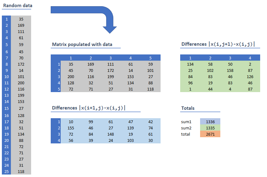Calculation of the objective

The grey matrix is just taking our original random data and lays them out row wise. The light blue matrix elements are the differences \(|x_{i+1,j}-x_{i,j}|\) while the light green area contains the differences: \(|x_{i,j+1}-x_{i,j}|\). The objective sums all these differences.

The idea is to find a different ordering of the data into the matrix such that the total sum of differences is minimized.

Trying out all permutations is not really feasible: \[25! =15511210043330985984000000\]

A first conceptual model

To distribute our numbers \(p_k\) to a matrix \(x_{i,j}\) we can use the concept of an assignment model:\[\begin{align}& \sum_{i,j} y_{k,i,j} = 1 &&\forall k \\ & \sum_k y_{k,i,j} = 1&&\forall i,j \\ & y_{k,i,j} \in \{0,1\} \end{align}\] The values can be recovered with \[x_{i,j} = \sum_k p_k y_{k,i,j}\] We used here the assignment model paradigm to implement a permutation of a data vector and place them in a matrix layout. The complete model can look like:

High-level model
\[\begin{align} \min & \sum_{i\lt n,j} \|\color{DarkRed} x_{i+1,j}-\color{DarkRed} x_{i,j}\| + \sum_{i,j \lt n} \|\color{DarkRed} x_{i,j+1}-\color{DarkRed} x_{i,j}\|\\ & \sum_{i,j} \color{DarkRed} y_{k,i,j} = 1 &&\forall k \\ & \sum_k \color{DarkRed} y_{k,i,j} = 1 &&\forall i,j \\ & \color{DarkRed}x_{i,j} = \sum_k \color{DarkBlue}p_k \color{DarkRed} y_{k,i,j} \\ & \color{DarkRed} y_{k,i,j} \in \{0,1\} \end{align} \]

High-level model

\[\begin{align} \min & \sum_{i\lt n,j} |\color{DarkRed} x_{i+1,j}-\color{DarkRed} x_{i,j}| + \sum_{i,j \lt n} |\color{DarkRed} x_{i,j+1}-\color{DarkRed} x_{i,j}|\\ & \sum_{i,j} \color{DarkRed} y_{k,i,j} = 1 &&\forall k \\ & \sum_k \color{DarkRed} y_{k,i,j} = 1 &&\forall i,j \\ & \color{DarkRed}x_{i,j} = \sum_k \color{DarkBlue}p_k \color{DarkRed} y_{k,i,j} \\ & \color{DarkRed} y_{k,i,j} \in \{0,1\} \end{align} \]

Note that I protected the terms of the objective against out-of-range indexing.

The original problem allowed the data vector \(p_k\) to have more elements than the matrix \(x_{i,j}\). This is easily fixed in our model. Rewrite the assignment constraints as: \[\begin{align} & \sum_{i,j} y_{k,i,j} \le 1 &&\forall k \\ & \sum_k y_{k,i,j} = 1 &&\forall i,j \end{align}\] In the following, I will focus on our sample data, which has the length of \(p_k\) equal to \(n^2\).

Linearization

This model can be easily linearized, e.g. by:

Linearized model
\[\begin{align} \min & \sum_{i\lt n,j} \color{DarkRed} d^d_{i,j} + \sum_{i,j \lt n} \color{DarkRed} d^r_{i,j}\\ & \sum_{i,j} \color{DarkRed} y_{k,i,j} = 1 &&\forall k \\ & \sum_k \color{DarkRed} y_{k,i,j} = 1 &&\forall i,j \\ & \color{DarkRed}x_{i,j} = \sum_k \color{DarkBlue}p_k \color{DarkRed} y_{k,i,j} \\ & - \color{DarkRed}d^d_{i,j} \le \color{DarkRed} x_{i+1,j}-\color{DarkRed} x_{i,j} \le \color{DarkRed}d^d_{i,j} &&\forall i\lt n,j \\ & - \color{DarkRed}d^r_{i,j} \le \color{DarkRed} x_{i,j+1}-\color{DarkRed} x_{i,j} \le \color{DarkRed}d^r_{i,j} &&\forall i,j\lt n \\ & \color{DarkRed} y_{k,i,j} \in \{0,1\} \\ & \color{DarkRed} d^d_{i,j}\ge 0,\color{DarkRed} d^r_{i,j}\ge 0 \end{align} \]

Linearized model

\[\begin{align} \min & \sum_{i\lt n,j} \color{DarkRed} d^d_{i,j} + \sum_{i,j \lt n} \color{DarkRed} d^r_{i,j}\\ & \sum_{i,j} \color{DarkRed} y_{k,i,j} = 1 &&\forall k \\ & \sum_k \color{DarkRed} y_{k,i,j} = 1 &&\forall i,j \\ & \color{DarkRed}x_{i,j} = \sum_k \color{DarkBlue}p_k \color{DarkRed} y_{k,i,j} \\ & - \color{DarkRed}d^d_{i,j} \le \color{DarkRed} x_{i+1,j}-\color{DarkRed} x_{i,j} \le \color{DarkRed}d^d_{i,j} &&\forall i\lt n,j \\ & - \color{DarkRed}d^r_{i,j} \le \color{DarkRed} x_{i,j+1}-\color{DarkRed} x_{i,j} \le \color{DarkRed}d^r_{i,j} &&\forall i,j\lt n \\ & \color{DarkRed} y_{k,i,j} \in \{0,1\} \\ & \color{DarkRed} d^d_{i,j}\ge 0,\color{DarkRed} d^r_{i,j}\ge 0 \end{align} \]

The variables \(d^d_{i,j}\) indicate the differences downward and the variables \(d^r_{i,j}\) are the differences when we look to the right.

This turns out to be a terribly difficult model to solve, even for our small data set. With a \(5 \times 5\) matrix we end up with \(25\times 25= 625\) binary \(y\) variables. This is normally a piece of cake for a good MIP solver. But, in fact, I was unable to solve this model to optimality with this data set by any MIP solver I tried. Even after several hours the gap was still substantial. We are in big, big trouble here.

We can add the extra constraint: \[ \sum_{i,j} x_{i,j} = \sum_k p_k\] This did not seem to make much difference.

A good initial solution

A simple heuristic is to sort the data and place the sorted \(p_k\) accordingly in the matrix. This gives a good initial solution, although it is not optimal.

Sorting gives a good initial solution

Non-decreasing values

In the above picture the values in the matrix were non-decreasing both row-wise and column wise, i.e. \[\begin{align} &x_{i,j} \le x_{i+1,j}\\ &x_{i,j} \le x_{i,j+1}\end{align}\] Intuitively, it makes sense to organize things like that. For a 1d vector this is somewhat obvious. For a 2d matrix things are a bit more complex, but it makes sense to start with the smallest value in the left upper corner cell \(x_{1,1}\), and end with the largest number in the right lower cell \(x_{n,n}\).

If we explicitly add the constraints that values \(x_{i,j}\) are both row wise and column wise non-decreasing, we achieve a number of things. First we can simplify the calculation of the differences:

Non-decreasing model
\[\begin{align} \min & \sum_{j} \color{DarkRed} d^d_{j} + \sum_{i} \color{DarkRed} d^r_{i} \\ & \sum_{i,j} \color{DarkRed} y_{k,i,j} = 1 &&\forall k \\ & \sum_k \color{DarkRed} y_{k,i,j} = 1 &&\forall i,j \\ & \color{DarkRed}x_{i,j} = \sum_k \color{DarkBlue}p_k \color{DarkRed} y_{k,i,j} \\ & \color{DarkRed}d^d_{j} = \color{DarkRed} x_{n,j}-\color{DarkRed} x_{1,j} && \forall j\lt n \\ & \color{DarkRed}d^r_{i} = \color{DarkRed} x_{i,n}-\color{DarkRed} x_{i,1} && \forall i\lt n\\ & \color{DarkRed}x_{i,j} \le \color{DarkRed}x_{i+1,j} && \forall i\lt n,j\\ & \color{DarkRed}x_{i,j} \le \color{DarkRed}x_{i,j+1} && \forall i,j\lt n\\ & \color{DarkRed} y_{k,i,j} \in \{0,1\} \\ & \color{DarkRed} d^d_{j}\ge 0,\color{DarkRed} d^r_{i}\ge 0 \end{align} \]

Non-decreasing model

\[\begin{align} \min & \sum_{j} \color{DarkRed} d^d_{j} + \sum_{i} \color{DarkRed} d^r_{i} \\ & \sum_{i,j} \color{DarkRed} y_{k,i,j} = 1 &&\forall k \\ & \sum_k \color{DarkRed} y_{k,i,j} = 1 &&\forall i,j \\ & \color{DarkRed}x_{i,j} = \sum_k \color{DarkBlue}p_k \color{DarkRed} y_{k,i,j} \\ & \color{DarkRed}d^d_{j} = \color{DarkRed} x_{n,j}-\color{DarkRed} x_{1,j} && \forall j\lt n \\ & \color{DarkRed}d^r_{i} = \color{DarkRed} x_{i,n}-\color{DarkRed} x_{i,1} && \forall i\lt n\\ & \color{DarkRed}x_{i,j} \le \color{DarkRed}x_{i+1,j} && \forall i\lt n,j\\ & \color{DarkRed}x_{i,j} \le \color{DarkRed}x_{i,j+1} && \forall i,j\lt n\\ & \color{DarkRed} y_{k,i,j} \in \{0,1\} \\ & \color{DarkRed} d^d_{j}\ge 0,\color{DarkRed} d^r_{i}\ge 0 \end{align} \]

Of course, with this assumption, we can fix \[\begin{align} & x_{1,1} = \min_k p_k \\ & x_{n,n} = \max_k p_k \end{align}\]

This model solves very fast, and we get the solution depicted above (marked by "optimal solution"). I believe this is the optimal solution for our overall problem, but I have not proven this mathematically.

A quadratic model

In the comments a different model is suggested:

Quadratic model
\[\begin{align} \min & \sum_{k,k'} \left[ \|\color{DarkBlue} p_k - \color{DarkBlue} p_{k'} \| \sum_{i,j} \left( \color{DarkRed}y_{k,i,j}\color{DarkRed}y_{k',i+1,j} + \color{DarkRed}y_{k,i,j}\color{DarkRed}y_{k',i,j+1} \right) \right] \\ & \sum_{i,j} \color{DarkRed} y_{k,i,j} = 1 &&\forall k \\ & \sum_k \color{DarkRed} y_{k,i,j} = 1 &&\forall i,j \\ & \color{DarkRed} y_{k,i,j} \in \{0,1\} \end{align} \]

Quadratic model

\[\begin{align} \min & \sum_{k,k'} \left[ |\color{DarkBlue} p_k - \color{DarkBlue} p_{k'} | \sum_{i,j} \left( \color{DarkRed}y_{k,i,j}\color{DarkRed}y_{k',i+1,j} + \color{DarkRed}y_{k,i,j}\color{DarkRed}y_{k',i,j+1} \right) \right] \\ & \sum_{i,j} \color{DarkRed} y_{k,i,j} = 1 &&\forall k \\ & \sum_k \color{DarkRed} y_{k,i,j} = 1 &&\forall i,j \\ & \color{DarkRed} y_{k,i,j} \in \{0,1\} \end{align} \]

Assume zeros when indexing out-of-range, i.e. \(y_{k,n+1,j}=y_{k,i,n+1}=0\). This model can be linearized manually (or this can be left to the solver: e.g. Cplex will linearized this automatically). Still not able to find a proven optimal solution in a short time.

A Constraint Programming formulation

Would a CP model help? First, the formulation can be very different than our MIP model:

We can use high-level global constraints such as all-different and element (use a variable as an index)
Everything is integer valued in our problem, which makes CP more viable,

Here is an attempt in Minizinc:

include "globals.mzn";

int: n=5;

int: n2=n*n;

array[1..n,1..n] of var int : indx;

array[1..n,1..n] of var int : x;

var int: z;

array[1..n2] of int: p;

p = [35,169,111,61,59,45,70,172,14,101,200,116,199,153,27,

128,32,51,134,88,72,71,27,31,118];

constraint forall (i,j in 1..n) (indx[i,j]>=1);

constraint forall (i,j in 1..n) (indx[i,j]<=n2);

constraint alldifferent([indx[i,j]|i,j in 1..n]);

constraint forall (i,j in 1..n) (x[i,j] = p[indx[i,j]]);

constraint z =

sum(i in 1..n-1,j in 1..n) (abs(x[i+1,j]-x[i,j])) +

sum(i in 1..n,j in 1..n-1) (abs(x[i,j+1]-x[i,j]));

solve minimize z;

The indx[i,j] array is a permutation of \(1,\dots,n^2\). This is easily implemented using the all-different constraint. This index array can be used to find the values \(x_{i,j}\) using the so-called element constraint: x[i,j] = p[indx[i,j]]. We use here a decision variable indx as an index of a data vector p.

Secondly, we need to solve this. Although the formulation was easy, solving this (small) problem is not trivial. The standard Minizinc solvers did not get close to our "optimal" solution.

Conclusion

The problem of populating a matrix with 25 numbers such that the difference between adjacent cells is minimized, turns out to be maddeningly difficult. Adding ordering conditions: values are non-decreasing row- and column-wise makes the model easy to solve. I don't believe we cut off the optimal solution with this, but I have no formal proof of this.

References

Algorithm to organize a matrix so that neighbors are closest, https://stackoverflow.com/questions/54216526/algorithm-to-organize-a-matrix-so-that-neighbors-are-closest

Yet Another Math Programming Consultant

Monday, January 21, 2019

Arranging a matrix