Linear Programming and Chebyshev Regression

The LAD (Least Absolute Deviation) or \(\ell_1\) regression problem (minimize the sum of the absolute values of the residuals) is often discussed in Linear Programming textbooks: it has a few interesting LP formulations [1]. Chebyshev or \(\ell_{\infty}\) regression is a little bit less well-known. Here we minimize the maximum (absolute) residual.

\[\bbox[lightcyan,10px,border:3px solid darkblue]
{\begin{align}\min_{\beta}\>&\max_i \> |r_i|\\
&y-X\beta = r\end{align}}\]

As in [1],  \(\beta\) are coefficients to estimate and  \(X,y\) are data. \(r\) are the residuals.
Some obvious and less obvious formulations are:

• Variable splitting:\[\begin{align}\min\>&z\\& z \ge  r^+_i + r^-_i\\&r^+_i - r^-_i =y_i –\sum_j X_{i,j}\beta_j\\&r^+_i, r^-_i\ge 0\end{align}\] With variable splitting we use two non-negative variables \(r^+_i - r^-_i\) to describe a value \(r_i\) that can be positive or negative. We need to make sure that one of them is zero in order for \(r^+_i + r^-_i\) to be equal to the absolute value \(|r_i|\). Here we have an interesting case, as we are only sure of this for the particular index \(i\) that has the largest absolute deviation (i.e. where \(|r_i|=z\)). In cases where \(|r_i|<z\) we actually do not  enforce \(r^+_i \cdot r^-_i = 0\). Indeed, when looking at the solution I see lots of cases where \(r^+_i > 0, r^-_i > 0\). Effectively those \(r^+_i,  r^-_i\) have no clear physical interpretation. This is very different from the LAD regression formulation [1] where we require all \(r^+_i \cdot r^-_i = 0\).
• Bounding:\[\begin{align}\min\>&z\\ & –z  \le y_i –\sum_j X_{i,j}\beta_j \le z\end{align}\]Here \(z\) can be left free or you can make it a non-negative variable (it will be non-negative automatically). Note that there are actually two constraints here: \(–z  \le y_i –\sum_j X_{i,j}\beta_j\) and \(y_i –\sum_j X_{i,j}\beta_j \le z\). This model contains the data twice, leading to a large number of nonzero elements in the LP matrix.
• Sparse bounding: This model tries to remedy the disadvantage of the standard bounding model by introducing extra free variables \(d\) and extra equations:\[\begin{align}\min\>&z\\ & –z  \le d_i \le z\\& d_i = y_i –\sum_j X_{i,j}\beta_j \end{align}\] Note again that \(–z  \le d_i \le z\) is actually two constraints: \(–z  \le d_i\) and \(d_i \le z\).
• Dual:\[\begin{align}\max\>&\sum_i y_i(d_i+e_i)\\&\sum_i X_{i,j}(d_i+e_i) = 0 \perp \beta_j\\&\sum_i (d_i-e_i)=1\\&d_i\ge 0, e_i\le 0\end{align}\]The estimates \(\beta\) can be found to be the duals of equation \(X^T(d+e)=0\).

We use the same synthetic data as in [1] with \(m=5,000\) cases, and \(n=100\) coefficients. Some timings with Cplex (default LP method) yield the following results (times are in seconds):



Opposed to the LAD regression example in [1], the bounding formulation is very fast here. The dual formulation remains doing very good.

Historical Note

The use of this minimax principle goes back to Euler (1749) [3,4].

Leonhard Euler (1707-1783)

The term Chebyshev regression is related to the Chebyshev distance (a different name for the \(\ell_{\infty}\) metric).

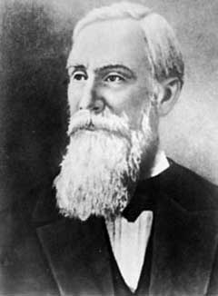
Pafnuty Lvovich Chebyshev (1821-1894)

References

1. Linear Programming and LAD Regression, http://yetanothermathprogrammingconsultant.blogspot.com/2017/11/lp-and-lad-regression.html
2. A.Giloni, M.Padberg, Alternative Methods of Linear Regression, Mathematical and Computer Modeling 35 (2002), pp.361-374.
3. H.L. Harter, The method of least squares and some alternatives, Technical Report, Aerospace Research Laboratories, 1972.
4. L. Euler, Pièce qui a Remporté le Prix de l'Academie Royale des Sciences en 1748, sur les Inegalités de Mouvement de Saturn et de Jupiter. Paris (1749).