Non-convex Quadratic Programming problems are difficult to solve to optimality. Most QP solvers do not even accept non-convex problems, so how can we attack this?
The easy way: global solvers
The easiest is just to use a global solver. We can use global NLP solvers such as Baron, Qouenne or Antigone. In addition Cplex has a solver for non-convex QP and MIQP problems (you need to set an option for this: OptimalityTarget = 3; Cplex will not automatically use this non-convex solver). For these solvers make sure to set the gap tolerance (GAMS option OPTCR) to zero.
Theory: KKT Conditions
A QP model can look like:
| \[\begin{align}\min\>\> & c^Tx + x^TQx \\ &Ax \le b\\ & \ell \le x \le u \end{align}\] |
The KKT conditions for this QP are:
| \[\begin{align} & 2Qx + c - A^T\mu – \lambda - \rho = 0\\ &(Ax – b)^T\mu = 0\\ &(x-\ell)^T\lambda = 0 \\ &(x-u)^T\rho = 0\\ & \ell \le x \le u \\ & Ax \le b \\ & \lambda \ge 0,\rho \le 0, \mu \le 0 \end{align}\] |
There are two complications with this LCP (Linear Complementarity Problem):
- The complementarity conditions \((Ax – b)^T\mu\), \((x-\ell)^T\lambda=0\) and \((x-u)^T\rho\) are not linear and can not be used directly in an LP or MIP model
- There are likely multiple solutions, so we need a way to select the best
A MIP formulation
To make the above model amenable to a linear solver we first try to linearize the complementarity conditions. Let’s consider \((x-\ell)^T\lambda=0\). This can be attacked as follows. The condition \((x_i –\ell_i)\lambda_i = 0\) really means \(x_i=\ell_i\) or \(\lambda_j=0\). This can be linearized as:
| \[\begin{align} & x_i \le \ell_i +M \delta_i\\ & \lambda_i \le M (1-\delta_i) \\ & \delta_i \in \{0,1\} \end{align}\] |
We can do something similar for \((x-u)^T\rho\) and \((Ax – b)^T\mu \).
The big-M coefficient are a problem of course. We either need to find some good values for them or use a formulation that does not need them. Some techniques that could help here are SOS1 (Special Order Sets of Type 1) variables where each combination \(y_i, \lambda_i\) (where \(y_i=x_i-\ell_i\) forms a SOS1 set. An alternative is to use some indicator variables (these are supported by a number of solvers).
The second issue is to find the best solution. Obviously we could add an objective \(\min\> c^Tx + x^TQx\) but that makes the problem non-linear again. It turns out that \(c^Tx + x^TQx = \frac{1}{2} \left[ c^Tx +\ell^T\lambda + u^T\rho+ b^T\mu\right]\). This is now a linear objective!
Objective
The derivation of the linear objective is as follows:
| \[\begin{align} & c^Tx + x^TQx\\ = \>& c^Tx + \frac{1}{2} x^T ( \lambda + \rho + A^T\mu – c)\\ = \> & c^Tx + \frac{1}{2}x^T\lambda + \frac{1}{2}x^T\rho + \frac{1}{2}(Ax)^T\mu – \frac{1}{2}x^Tc\\ =\> & \frac{1}{2} c^Tx + \frac{1}{2}\ell^T\lambda + \frac{1}{2}u^T\rho + \frac{1}{2} b^T\mu \end{align}\] |
It is quite fortunate that we are able to get rid of the quadratic term and form a linear objective.
Example: Non-convex QP
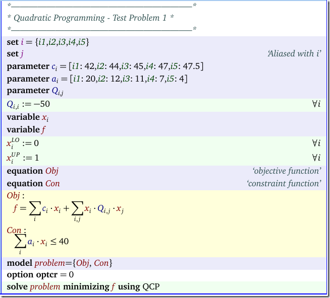
A simple example is from (1):
Solving this directly gives:
| LOWER LEVEL UPPER MARGINAL ---- EQU Obj . . . 1.0000 Obj objective function ---- VAR x LOWER LEVEL UPPER MARGINAL i1 . 1.0000 1.0000 -58.0000 LOWER LEVEL UPPER MARGINAL ---- VAR f -INF -17.0000 +INF . |
Example: MIP with big-M coefficients
We name our duals as follows:
| \[\begin{align} x_i \ge \ell_i & \perp \lambda_i \ge 0 \\ x_i \le u_i & \perp \rho_i \le 0 \\ \sum_i a_i x_i \le b & \perp \mu \le 0 \end{align}\] |
The complete model looks like:
The results look like:
| LOWER LEVEL UPPER ---- VAR f -INF -17.0000 +INF ---- VAR x LOWER LEVEL UPPER i1 . 1.0000 1.0000 ---- VAR lambda dual of x.lo LOWER LEVEL UPPER i1 . . +INF ---- VAR rho dual of x.up LOWER LEVEL UPPER i1 -INF -58.0000 . LOWER LEVEL UPPER ---- VAR mu -INF . . mu dual of a*x<=b ---- VAR delta LOWER LEVEL UPPER lo.i1 . 1.0000 1.0000 LOWER LEVEL UPPER ---- VAR gamma . 1.0000 1.0000 |
For some performance comparisons see (3).
References
(1) Floudas e.a., Handbook of Test Problems in Local and Global Optimization, Kluwer, 1999.
(2) Wei Xia, Juan Vera, Louis F. Zuluaga, Globally Solving Non-Convex Quadratic Programs via Linear Integer Programming Techniques, report, Nov 17, 2015.
(3) http://yetanothermathprogrammingconsultant.blogspot.com/2016/07/non-convex-qp-as-mip-performance.html


Thanks :))
ReplyDelete