Page rank in GAMS

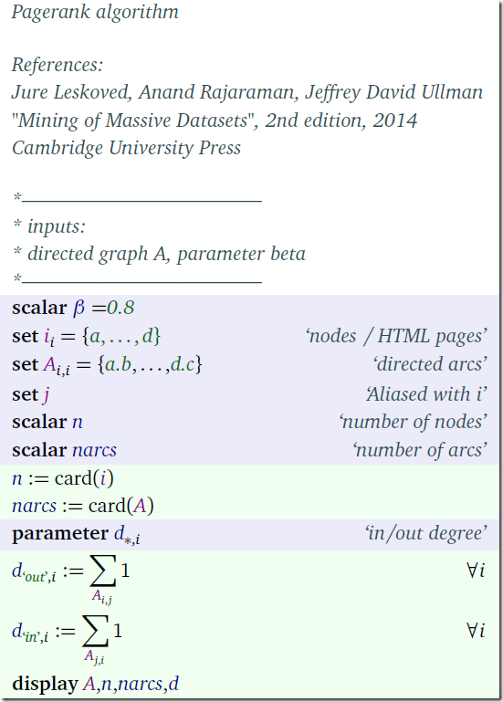
The Google PageRank algorithm is a well known algorithm to calculate web page rankings in a search engine. It is surprisingly simple (for smaller data sets). The basic update equation for the page rank estimate v looks like:

We iterate this thing until the v’s converged. Note that in GAMS this is a parallel assignment so we don’t need to worry about v’s being overwritten during the assignment (otherwise we could have used vprev in the right-hand side expression, see further below). To test this we first load the (sparse) matrix and calculate the degree of each node:

The actual algorithm should perform quite reasonable in GAMS as we can exploit the sparse execution of the matrix-vector multiplication inside the loop. Note that the transition matrix M is transposed wrt A. The loop terminates as soon as the update does not change v anymore.

Indeed I was able to run this model quickly even with the harvard500 data set (http://www.mathworks.com/moler/exm/chapters/pagerank.pdf). For this 500 node web graph the loop takes about 0.5 seconds.

Note: parallel assignment

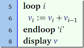
The detail about the parallel assignment can be illustrated with:

In line 4 we set v := [1,2,3,…,10]. After line 5 we have (using parallel assignment): v = [1,2,5,…,19]. If we would have executed:

then we see a result of: v = [1,3,6,…,55].

GAMS vs Matlab

There is no solve in the GAMS code, so Matlab should do very well on this also. In Matlab we can even compare dense vs sparse execution (GAMS always uses sparse storage).

GAMS Sparse M Time: 0.5 s Iterations: 28	loop(iter$(sum(i,abs(v(i)-vprev(i)))>epsilon),    vprev(i)=v(i);    v(i) = beta*sum(j, M(i,j)*v(j)) + (1-beta)/n; );
MATLAB Dense M Time: 0.03 s Iterations: 28	for iter=1:100    vprev=v;    v = beta*M*v + (1-beta)/n;    if (norm(v-vprev,1)<epsilon)        break;    end; end
MATLAB Sparse M Time: 0.01 s Iterations: 28

We can see Matlab is doing much better on the matrix-vector products especially when using a sparse matrix M. The difference between sparse and dense should increase for larger matrices: 500x500 is actually not that big and works quite well with dense linear algebra. The density of the M matrix is 1% in this example and should be smaller for larger matrices. Matlab is very fast as long as we can use the computational kernels efficiently, which is the case here.

Complete code

Here we show the complete model. As it turns out the loop looks quite similar, but some of the initialization code is really different between GAMS and Matlab. Matlab is of course much closer to real mathematical notation than GAMS. I am not sure this always helps in making code more readable. This small example actually shows this succinctly.

GAMS	MATLAB
scalar beta /0.8/; set i 'nodes / HTML pages' /a,b,c,d/; alias(i,j) set a(i,j) 'directed arcs' /   a.(b,c,d)   b.(a,d)   c.c   d.(b,c) /;	beta = 0.8; i = [1,1,1,2,2,3,4,4]; j = [2,3,4,1,4,3,2,3]; A = sparse(i,j,ones(size(i,2),1));
Here we load the data. In GAMS we index over sets consisting of strings. Typically a network graph is implemented as two sets: a one dimensional set with nodes and a two dimensional set with arcs. In Matlab we use matrices where we index over integers 1..n. Here we specify a sparse matrix by providing the row and column numbers; the nonzero values are all one. I prefer the GAMS representation of the graph.
scalars   n   'number of nodes'   narcs  'number of arcs' ; n = card(i); narcs = card(a); parameter d(*,i) 'in/out degree'; d('out',i) = sum(a(i,j),1); d('in',i) = sum(a(j,i),1); display a,n,narcs,d;	n=size(A,1); narcs=nnz(A); d_in = sum(A,1); d_out = sum(A,2);
GAMS needs more lines of code because all identifiers need to be declared before they can be used. This is cumbersome for interactive use but provides extra protection for larger projects. Also GAMS is basically a batch environment (there is no console where we type GAMS commands). GAMS is a very small language. In this model we basically only use the sum operator and the card and abs functions. Matlab has a very rich set of matrix functions (we use here sparse, ones, size, nnz, sum, find, norm). That is of course both a blessing and a curse: we can write things down very compactly but you need to know more stuff before being proficient in Matlab.
set iter /iter1*iter100/; scalars    epsilon 'convergence tolerance' /1e-5/ ; parameter    M(i,j) 'transition matrix j->i'    v(i) 'page rank'    vprev(i) 'page rank from previous iteration' ; * initialization M(i,j)$a(j,i) = 1/d('out',j); display M; v(i) = 1/n; vprev(i) = 0; loop(iter$(sum(i,abs(v(i)-vprev(i)))>epsilon),    vprev(i)=v(i);    v(i) = beta*sum(j, M(i,j)*v(j)) + (1-beta)/n;    display v; ); display v;	epsilon=1.0e-5; k = find(d_out~=0); D = sparse(k,k,1./d_out(k),n,n); M = A' * D; v = ones(n,1)/n; for iter=1:100     vprev=v;     v = beta*M*v + (1-beta)/n;     if (norm(v-vprev,1)<epsilon)          break;     end    end
The construction of the transition matrix M is cleaner in GAMS than in Matlab. It may not be immediately obvious but in the Matlab code the matrix D is a diagonal matrix. Of course we want to store this sparse. The use of a diagonal matrix in Matlab is a well-known trick to keep things vectorized (opposed to using explicit loops). Explicit loops are often bad (i.e. slow) both in GAMS and in Matlab (often beginners tend to overuse loops in both languages). The major iteration loop is programmed in such a way that it always terminates (either by convergence or running out of iterations). This is a useful defensive approach. The test for convergence can be embedded in the loop statement in GAMS (note that this requires vprev to be initialized at this point). In Matlab there is no such trick so we just do the test at the most convenient place. Finally note the difference in the display of the graph A. Arguably the GAMS output is a little bit better to understand. We can improve the Matlab output by saying display(full(A)). Of course we only should do a display of a small graph.
----     38 SET a  directed arcs             a           b           c           d a                     YES         YES         YES b         YES                                 YES c                                 YES d                     YES         YES	>> display(A) A =    (2,1)        1    (1,2)        1    (4,2)        1    (1,3)        1    (3,3)        1    (4,3)        1    (1,4)        1    (2,4)        1

Convergence

The convergence of the term sum(abs(v-vprev)) is interesting. We plot here against the iteration number:

With a logarithmic scale: