Gurobi vs R: subset selection

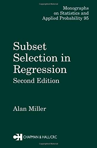
The R package leaps (http://cran.r-project.org/web/packages/leaps/leaps.pdf) provided a convenient way to perform feature selection. The methods are based on work by Alan Miller, described in:

Alan Miller, “Subset Selection in Regression”, Chapman and Hall/CRC; 2 edition (April 15, 2002)

In a related paper: Alan Miller, “Subsets of Regression Variables”, J. R. Statist. Soc. A (1984), 147, Part 3, pp. 389-425 (http://citeseerx.ist.psu.edu/viewdoc/download?doi=10.1.1.474.3223&rep=rep1&type=pdf) we even see some comments from Beale.

We should be able to reproduce the “exhaustive” method from the leaps package using an MIQP formulation. Something like:

 

Given a value for n we want to minimize SSQ. The binary variables δ indicate whether a feature j can appear in the model (we exclude the constant term: that one remains in the model). We need to solve this model for n=1,2,3,… To be complete, the other symbols are β: the quantities we want to estimate, data X,y and our big M constant.

I would guess that say Gurobi would do a better job than leaps. As it turns out, it was not easy to beat leaps.

To generate a random model we use a very simplistic scheme. Not sure if this has much in common with real world data sets, but a similar approach was used in Gatu, Kontoghiorghes, “Branch-and-Bound Algorithms for Computing the Best-Subset Regression Models”, Journal of Computational and Graphical Statistics, Volume 15, Number 1, Pages 139–156:

We use N=50 variables in total of which we want to select n=1,2,3,..,10 variables.

GAMS/Gurobi

Here are the results:

----     87 PARAMETER t                    =      112.897  elapsed time of solve loop ----     87 SET selected  selected variables              v5          v6          v8         v11         v13         v19         v31         v32         v35 n1                      YES n2                      YES n3                      YES                                                         YES n4                      YES                                                         YES n5                      YES                                             YES         YES n6                      YES                                             YES         YES                     YES n7                      YES         YES                                 YES         YES                     YES n8                      YES         YES                     YES         YES         YES                     YES n9                      YES         YES                     YES         YES         YES         YES         YES n10         YES         YES         YES         YES         YES         YES         YES                     YES   +         v40         v43 n2          YES n3          YES n4          YES         YES n5          YES         YES n6          YES         YES n7          YES         YES n8          YES         YES n9          YES         YES n10         YES         YES ----     87 PARAMETER rss  residual sum of squares n1  836.651,    n2  836.342,    n3  836.060,    n4  835.869,    n5  835.677,    n6  835.495,    n7  835.330 n8  835.189,    n9  835.075,    n10 834.937 ----     87 PARAMETER solvetime  time for each solve n1   0.080,    n2   0.135,    n3   0.609,    n4   1.951,    n5   3.876,    n6   6.878,    n7  15.971,    n8  21.016 n9  30.122,    n10 27.511

A few notes:

• The model is very sensitive to the size of M. I used M=1000. With M=1e5 we get into trouble. We can see messages like: Warning: max constraint violation (1.2977e-02) exceeds tolerance (possibly due to large matrix coefficient range).This QP formulation is not so easy to solve for Gurobi from a numerical standpoint.
• The RSS is going down when we add variables. As expected.
• Also as expected: the time to solve each sub-problem goes up when we have more variables in the model. “pick n out of N”  constructs often cause performance problems.
  
• I used a small optcr (gap) and 4 threads to make Gurobi fast enough to beat Leaps. (Leaps takes 3 minutes and a loop of 10 solves with Gurobi takes 2 minutes).
• I often like to formulate a separate fit equation as in:
  
  This turns out to be very bad w.r.t. performance. Of course the fit equation forms a completely dense block in the coefficient matrix, something Gurobi was not designed for (it likes sparse structures much better).

R/Leaps

The R code is simply:

d<-dbGetQuery(db,"select * from data") %>% dcast(i ~ v) %>% select(-i)
system.time(r <- regsubsets(y~.,data=d,nvmax=10,really.big=T))

The first line gets the data from the database and applies a pivot operation (from a long, skinny data frame with three columns i,v,value to a wide one with 10 columns v1,v2,v3,…,v10). This trick is useful to remember is this happens a lot when reading data from a database (such data is typically organized in long, skinny tables opposed to a “matrix” organization). The second line calls the regsubsets function from the Leaps package.

The output is:

v1 v10 v11 v12 v13 v14 v15 v16 v17 v18 v19 v2 v20 v21 v22 v23 v24 v25 v26 v27 v28 1 ( 1 ) " " " " " " " " " " " " " " " " " " " " " " " " " " " " " " " " " " " " " " " " " " 2 ( 1 ) " " " " " " " " " " " " " " " " " " " " " " " " " " " " " " " " " " " " " " " " " " 3 ( 1 ) " " " " " " " " " " " " " " " " " " " " " " " " " " " " " " " " " " " " " " " " " " 4 ( 1 ) " " " " " " " " " " " " " " " " " " " " " " " " " " " " " " " " " " " " " " " " " " 5 ( 1 ) " " " " " " " " " " " " " " " " " " " " "*" " " " " " " " " " " " " " " " " " " " " 6 ( 1 ) " " " " " " " " " " " " " " " " " " " " "*" " " " " " " " " " " " " " " " " " " " " 7 ( 1 ) " " " " " " " " " " " " " " " " " " " " "*" " " " " " " " " " " " " " " " " " " " " 8 ( 1 ) " " " " " " " " "*" " " " " " " " " " " "*" " " " " " " " " " " " " " " " " " " " " 9 ( 1 ) " " " " " " " " "*" " " " " " " " " " " "*" " " " " " " " " " " " " " " " " " " " " 10 ( 1 ) " " " " "*" " " "*" " " " " " " " " " " "*" " " " " " " " " " " " " " " " " " " " " v29 v3 v30 v31 v32 v33 v34 v35 v36 v37 v38 v39 v4 v40 v41 v42 v43 v44 v45 v46 v47 1 ( 1 ) " " " " " " " " " " " " " " " " " " " " " " " " " " " " " " " " " " " " " " " " " " 2 ( 1 ) " " " " " " " " " " " " " " " " " " " " " " " " " " "*" " " " " " " " " " " " " " " 3 ( 1 ) " " " " " " "*" " " " " " " " " " " " " " " " " " " "*" " " " " " " " " " " " " " " 4 ( 1 ) " " " " " " "*" " " " " " " " " " " " " " " " " " " "*" " " " " "*" " " " " " " " " 5 ( 1 ) " " " " " " "*" " " " " " " " " " " " " " " " " " " "*" " " " " "*" " " " " " " " " 6 ( 1 ) " " " " " " "*" " " " " " " "*" " " " " " " " " " " "*" " " " " "*" " " " " " " " " 7 ( 1 ) " " " " " " "*" " " " " " " "*" " " " " " " " " " " "*" " " " " "*" " " " " " " " " 8 ( 1 ) " " " " " " "*" " " " " " " "*" " " " " " " " " " " "*" " " " " "*" " " " " " " " " 9 ( 1 ) " " " " " " "*" "*" " " " " "*" " " " " " " " " " " "*" " " " " "*" " " " " " " " " 10 ( 1 ) " " " " " " "*" "*" " " " " "*" " " " " " " " " " " "*" " " " " "*" " " " " " " " " v48 v49 v5 v50 v6 v7 v8 v9 1 ( 1 ) " " " " " " " " "*" " " " " " " 2 ( 1 ) " " " " " " " " "*" " " " " " " 3 ( 1 ) " " " " " " " " "*" " " " " " " 4 ( 1 ) " " " " " " " " "*" " " " " " " 5 ( 1 ) " " " " " " " " "*" " " " " " " 6 ( 1 ) " " " " " " " " "*" " " " " " " 7 ( 1 ) " " " " " " " " "*" " " "*" " " 8 ( 1 ) " " " " " " " " "*" " " "*" " " 9 ( 1 ) " " " " " " " " "*" " " "*" " " 10 ( 1 ) " " " " " " " " "*" " " "*" " " user system elapsed 194.41 0.00 194.44 > summary(r)$rss [1] 836.6514 836.3416 836.1431 835.9519 835.7598 835.5764 835.4079 835.2662 835.1392 835.0116

The sum of squares start out the same but they diverge just a little bit.

The selected variables are much the same as using Gurobi (but there are a few differences here and there). The time is actually close to that of Gurobi. This performance is much better than I expected.