More on network models

I received some additional questions on solving some very large network models. Basically we used the formulation presented here: http://yetanothermathprogrammingconsultant.blogspot.com/2011/06/network-formulation.html. A slightly more optimized version is shown below:

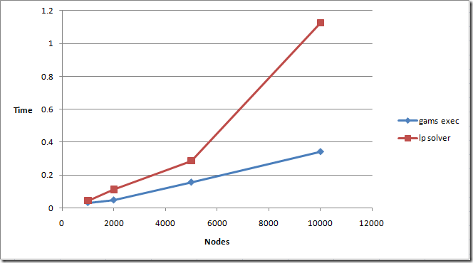
$ontext   large sparse max flow network example   Performance       nodes  arcs    gams       solver                      execution  time       1k     10k     0.031      0.045       2k     20k     0.047      0.112       5k     50k     0.156      0.286       10k   100k     0.343      1.125   Erwin Kalvelagen,   Amsterdam Optimization,   erwin@amsterdamoptimization.com $offtext $set n 10000 option limrow=0, limcol=0, solprint=off; sets   i   source(i)   sink(i) ; alias(i,j); parameter capacity(i,j) 'capacity, but also defines network'; $gdxin network%n% $loaddc i source sink capacity abort$(card(source)<>1) "We want one source node"; abort$(card(sink)<>1) "We want one sink node"; set arcs(i,j) 'we have an arc if capacity<>0'; arcs(i,j)$capacity(i,j) = yes; scalar narcs 'number of arcs'; narcs = card(arcs); display narcs; parameter rhs(i); rhs(source) = -1; rhs(sink) = 1; variables   x(i,j) 'flow along arcs'   f      'total flow' ; positive variables x; x.up(arcs) = capacity(arcs); equations    flowbal(i) 'flow balance' ; flowbal(i)..    sum(arcs(j,i), x(j,i)) - sum(arcs(i,j), x(i,j)) =e= f*rhs(i); model m /flowbal/; solve m maximizing f using lp; display f.l;

The performance of GAMS looks very good. GAMS execution time scales slightly better than the LP solver used to solve the problem:

GAMS almost scales linearly with the number of nonzero elements to be generated. In this case that means linearly with the number of nodes (because the number of nonzeroes is equal to 10*nodes in these models).

The main difference with the earlier model is that we replaced:

x.up(i,j) = capacity(i,j);

by

x.up(arcs) = capacity(arcs);

This actually saves some time and memory. In the first case we set many x.up’s to zero even though they are not used in the model. These variables with non-default bounds will need to be created and use up memory. In the second case, we only touch variables that are really used.

This small change makes a lot of difference for larger models. For n=5k we see GAMS execution time decrease from 3.775 seconds to 0.156 seconds. If things get large one needs to pay attention to detail!

AMPL Version

A direct translation to AMPL can look like:

set nodes; set source within nodes; set sink within nodes; param capacity {(i,j) in (nodes cross nodes)}, default 0; set arcs within (nodes cross nodes) := {i in nodes, j in nodes: capacity[i,j]}; # version 1 : slow calc of arcs # set arcs := {i in nodes, j in nodes: capacity[i,j]};                                   # version 2 : slow calc of x # set arcs within (nodes cross nodes);                                                    # version 3 : fast, read from data file param rhs{i in nodes} := if i in source then -1 else if i in sink then +1; var x {(i,j) in arcs} >= 0, <= capacity[i,j]; var f; maximize obj:f; subject to flowbal{i in nodes}:    sum{(j,i) in arcs} x[j,i] - sum{(i,j) in arcs} x[i,j] = f*rhs[i];

This formulation is not handled very efficiently by AMPL: the timings for n=5k are

##genmod times: ##seq      seconds    cum. sec.    mem. inc.  name ## 77            0            0            0  derstage ## 81            0            0            0  sstatus ## 95            0            0            0  nodes ## 96            0            0            0  source ## 97            0            0            0  sink ## 98            0            0            0  capacity ## 99      10.4521      10.4521   1146012664  arcs ## 100            0      10.4521            0  rhs ## 101    0.0156001      10.4677        65544  x ## 103            0      10.4677            0  f ## 105            0      10.4677            0  obj ## 107    0.0624004      10.5301      4148296  flowbal

Especially the calculation of the set arcs is expensive.

Note that if we use an alternative for arcs:

set arcs := {i in nodes, j in nodes: capacity[i,j]};

the burden is moved to x:

##genmod times: ##seq      seconds    cum. sec.    mem. inc.  name ## 77            0            0            0  derstage ## 81            0            0            0  sstatus ## 95            0            0            0  nodes ## 96            0            0            0  source ## 97            0            0            0  sink ## 98            0            0            0  capacity ## 99            0            0            0  arcs ## 100            0            0            0  rhs ## 101      10.5301      10.5301   1147323392  x ## 103            0      10.5301            0  f ## 105            0      10.5301            0  obj ## 107    0.0780005      10.6081      4147928  flowbal

When we run a few different instances we see we do something causing non-linear scaling:

It is clear this is not a good approach. We need to do something about this set arcs. In AMPL we don’t really need to calculate this set, we can directly populate this from the data by replacing in the data file:

param: capacity := n1 n32 87 n1 n37 44 n1 n124 38 …

by

param: arcs : capacity := n1 n32 87 n1 n37 44 n1 n124 38 …

Now we get the set arcs basically for free, and we get linear scaling:

The total AMPL generation time vs. LP solution time is here:

This is very close to the GAMS timings given that this was on a different machine.

GLPK

The open source tool GLPK can handle many AMPL linear models. However, in some cases it is substantial slower. This model demonstrates this behavior. We run the model as:

C:\projects\tmp>timeit \Projects\glpk\glpk\bin\glpsol.exe -m network.mod -d network1000.dat Reading model section from network.mod... network.mod:24: warning: unexpected end of file; missing end statement inserted 24 lines were read Reading data section from network1000.dat... network1000.dat:10108: warning: unexpected end of file; missing end statement inserted 10108 lines were read Generating obj... Generating flowbal... Model has been successfully generated lpx_simplex: original LP has 1001 rows, 10001 columns, 20003 non-zeros lpx_simplex: presolved LP has 1000 rows, 10001 columns, 20002 non-zeros lpx_adv_basis: size of triangular part = 999 *     0:   objval =  0.000000000e+000   infeas =  0.000000000e+000 (1) *   171:   objval =  4.780000000e+002   infeas =  0.000000000e+000 (1) OPTIMAL SOLUTION FOUND Time used:   0.1 secs Memory used: 13.4M (14073536 bytes) Version Number:   Windows NT 6.0 (Build 6002) Exit Time:        0:32 am, Thursday, August 4 2011 Elapsed Time:     0:00:05.563 Process Time:     0:00:05.600 System Calls:     160954 Context Switches: 89933 Page Faults:      20453 Bytes Read:       248437 Bytes Written:    87315 Bytes Other:      130434 C:\projects\tmp>

Besides being much slower than AMPL, the performance of the model generation phase is showing more than linear scaling:

Model generation is here calculated as total elapsed time minus time used for the LP solver.

My conclusions:

1. AMPL and GAMS are capable of generating simple network models faster than a good LP solver can solve them
2. But a simple mistake and performance goes down the drain
3. Direct translations between GAMS and AMPL models are not always a good idea.