Suguru

Suguru is another popular, Sudoku-like puzzle originating from Japan.

 

We need to fill every block with unique numbers \(1,2,..,n_b\) where \(n_b\) is the number of cells in a block. (This implies a singleton block – a block with just one cell – has to contain the value 1. In the puzzle above, the two singleton blocks are already filled in. I am not sure why.) The constraint is that neighboring cells can not contain the same number. Here a neighbor includes the cell diagonally touching (i.e., an interior cell has 8 neighbors).

To solve this as a MIP model, as usual for these type of puzzles (see [2]), we can define our binary decision variable as:

\[x_{i,j,k}=\begin{cases}1 &\text{if cell \((i,j)\) has value $k$}\\ 0 & \text{otherwise}\end{cases}\]

Here \(k\) is running from \(1,\dots,n_b\), i.e. it depends on the block \(b\) containing cell \((i,j)\) . Some of these values can be fixed using the initially given values:

\[x_{i,j,k} = 1 \>\text{if $V^0_{i,j}=k$}\]

where \(V^0\) are the provided initial values.

Of course only one value can be selected in a cell:

\[\sum_{k=1}^{n_b} x_{i,j,k} = 1\>\>\forall i,j\]

In the following we assume we have a map \(B_{b,i,j}\) which is true if cell \((i,j)\) is in block \(b\). The uniqueness within a block is not very difficult to establish:

\[\sum_{i,j|B_{b,i,j}} x_{i,j,k} = 1 \>\>\>\begin{align}&\forall b\\ &\forall k\le n_b\end{align}\]

Again, only applicable \(k\)'s are to be considered.

Finally, we need to make sure neighboring cells do not have the same value as cell \((i,j)\). One way to handle this, is to have a large number of pairwise constraints:

\[x_{i,j,k}+x_{i’,j’,k}\le 1\>\>\> \begin{align}&\forall (i,j),(i’,j’) | N_{i,j,i’,j’}\\ &\forall k \le \min\{n_b,n_{b’}\}\end{align}\]

Here \(N_{i,j,i',j'}\) indicates whether cells \((i,j)\) and \((i',j')\) are neighbors. We can restrict this to neighbors that are in different blocks only (we already compared values in the same block). In addition we can cut the number of these constraints in half by observing that if we compared cells \((i,j)\) and \((i',j')\) we do not have to check \((i’,j’)\) and \((i,j)\). (See [3] for a similar symmetry issue.) Also we can restrict \(k\) to the smallest value \(\min\{n_b,n_{b’}\}\) where \((i,j\)) is in \(b\) and \((i’,j’)\) is in \(b’\). This constraint needs some attention if you want to prevent generating unnecessary pairs. 

If you would be generous and ignore all these points you would generate \(\mathit{NumNeigbors} \times \max n_b = 2375\) of these pairwise equations. Being stingy, we can reduce this to \(503\) equations.

To display a solution we can calculate:

\[v_{i,j} = \sum_k k \cdot x_{i,j,k}\]

We can do this outside the model using the solution values of \(x\), or we can add a reporting equation to the model (this is sometimes called an “accounting row”) and let the solver calculate the \(v\) values for us.

There is no objective: we just want to find a feasible solution.

A good solver will say something like:

MIP Presolve eliminated 630 rows and 298 columns.
All rows and columns eliminated.

I.e. the presolve completely solves the model and we don’t have to do any branching.

The solution looks like:

The solution is unique. We can get some hard evidence of that by taking this solution \(s_{i,j,k}=x^*_{i,j,k}\) and adding the constraint:

\[\sum_{i,j,k} s_{i,j,k} x_{i,j,k} \le n-1\]

where \(n\) is the number of cells. If we resolve the problem, the model is declared infeasible. This confirms there is only one, unique solution.

Conclusion

Even though this initially looked like a simple problem that can be easily modeled as a MIP problem, there are some interesting wrinkles. This modeling approach is very different from writing an algorithm [1].   

References

1. Solving Suguru (Tectonic) puzzles, http://community.wolfram.com/groups/-/m/t/1077888. Contains Matlab code to solve the puzzle. The above example was taken from this document.
2. MIP Modeling: from Sudoku to KenKen via Logarithms, http://yetanothermathprogrammingconsultant.blogspot.com/2016/10/mip-modeling-from-sudoku-to-kenken.html
3. No overlapping jobs, http://yetanothermathprogrammingconsultant.blogspot.com/2017/10/no-overlapping-jobs.html
4. Suguru: GAMS/MIP vs Python/Z3, http://yetanothermathprogrammingconsultant.blogspot.com/2017/11/suguru-gamsmip-vs-pythonz3.html. Compare code in GAMS and Python using a MIP and a Z3 formulation. Conclusion: the data manipulation is more complex than the model constraints themselves.

no overlapping jobs

A standard problem in continuous time job-scheduling is to forbid jobs to overlap:

\[\begin{align}&S_i \ge E_j\\ &\text{or}\\ &S_j \ge E_i\end{align}\]

where \(S_i\) and \(E_i\) are start and finishing times of job \(i\):

In a MIP this is usually formulated as [1]:

\[\begin{align}&S_i\ge E_j - M\delta_{i,j}\\ &S_j \ge E_i - M(1-\delta_{i,j})\\ &\delta_{i,j} \in \{0,1\}\end{align}\]

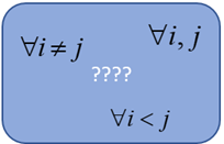
Best choice: \(\forall i<j\)

If we compare job \(i\) with \(j\), we no longer need to check job \(j\) and \(i\). So often we implement the constraints only for the combinations \(i<j\) (of course \(\forall j>i\) would be just as valid).

In this post I want to investigate a bit what happens if we choose a different set of combinations over which we apply the constraints.

Case 2: \(\forall i,j\)

What happens if we are sloppy with this and compare for all \(i,j\)? If \(i=j\), we introduce an infeasibility that is easily detected by the solver. Some solvers do report:

Model is infeasible or unbounded

which is a little bit less helpful. In any case, the model will not solve if the modeler applies these constraints for all \(i,j\).

Case 3: \(\forall i\ne j\)

Now, what happens if we use \(\forall i\ne j\) instead of \(\forall i<j\)? This is actually something I see quite often in models (see [2] for an example). The solver (or modeling system) will not provide any feedback on this. It will solve the model and provides correct solutions in both cases.

What about solution times? There are two things to consider:

1. The number of binary variables \(\delta_{i,j}\) increases two-fold. However, implicitly the model enforces \(\delta_{i,j}=1-\delta_{j,i}\). If a variable \(\delta_{i,j}\) is fixed to zero or one, automatically \(\delta_{j,i}\) will also assume an integer value. The total impact of this on the node count of MIP solver is not clear to me. Indeed, the number of nodes is not uniformly better using either formulations.
2. The number of equations (and variables) involved increases by a factor of 2. This should slow down the LP relaxations solved by the MIP solvers. I would expect the speed in terms of the number of nodes per second or Simplex iterations per second to decrease. This turns out to be an important factor.

Let’s try this out on a smallish but difficult job shop problem [3].

Indeed we see no consistency in the node count. However the number of nodes per second and iterations per second behaved as I predicted. The total time is affected by this in such a manner that the funny difference in node count is not as significant as the difference in speed solving the LP relaxations. Even in cases where the node count or iteration count is better for the \(i\ne j\) model, it still loses out on total time. I.e. \(i<j\) is a winner, but may be for a different reason than you might think.

Conclusion: please use \(i<j\) when implementing the no-overlap equations.

References

1. Alan Manne, On the job-shop scheduling problem, Operations Research, Vol. 8, No. 2, March-April 1960.
2. ojAlgo Linear Optimization - Preventing work shift overlaps?, https://stackoverflow.com/questions/46823121/ojalgo-linear-optimization-preventing-work-shift-overlaps. I am not familiar with ojAlgo, but the presented model in the answer does seem to implement just \(i \ne j\).
3. Data set ft10 from H. Fisher, G. L. Thompson, Probabilistic learning combinations of local job-shop scheduling rules, in: J. F. Muth, G. L. Thompson (eds.),  Industrial Scheduling, Prentice Hall, Englewood Cliffs, N.J., 1963.

Profiling in visual studio

Somehow, I am often struggling to understand the output of profilers. This report of Visual Studio actually makes sense to me:

I like the code highlighting. It gives a really quick overview of where most of the time is spent. (Most of the time in parsing some files is spent in dealing with the regular expression; I am happy: no obviously poor performance somewhere in my code. Interestingly, also when parsing the Excel formulas I spent most of the time parsing Excel addresses – again using a regular expression.)

“Coda is a next-generation spreadsheet designed to make Excel a thing of the past”

Picture from [4]

Not so easy in my opinion. Excel is the workhorse in many workplaces.

1. https://www.theverge.com/2017/10/19/16497444/coda-spreadsheet-krypton-shishir-mehrotra (the title is from this post).
2. https://coda.io/welcome
3. https://blog.coda.io/
4. https://en.wikipedia.org/wiki/Spreadsheet

Pareto fronts in Z3: a large data set

In [1] a small multi-objective MIP is solved with Z3. Here we try a larger problem, an engineering design problem. It has three objectives and 2029 non-dominated solutions. The solution in the F space (the objectives) looks like:

To make life easier for Z3, I converted the objectives to integer values. The good news is that Z3 finds the same number of solutions. The bad news: for this problem it is not very fast:

We see it is getting slower and slower:

The first 500 solutions are found in a rate of about a second per solution. Later on this becomes 10 seconds per solution.

Brute force

A brute force method for this problem is:

1. Generate all feasible integer solutions for this problem. I used Cplex for this, using the solution pool technology. I get about 4.8 million solutions.
2. Filter out all dominated solutions. There are 2029 remaining non-dominated solutions.

This method takes about 20 minutes (i.e. 1200 seconds).

References

1. http://yetanothermathprogrammingconsultant.blogspot.com/2017/10/multi-objective-mixed-integer.html

Multi-objective Mixed Integer Programming and Z3

Vilfredo Federico Damaso Pareto (1848-1923) [link]

The tool \(\nu Z\) [1,2] is an optimization extension to the SMT solver Z3 [3]. It can actually generating Pareto optimal solutions for MIP problems, using an algorithm based on [6]. In [4,5] a small example model is presented:

\[\bbox[lightcyan,10px,border:3px solid darkblue]{ \begin{align}\max\>&x_1 – 2x_2\\ \max\>&-x_1+3x_2\\ &x_1 \le 2x_2\\ &x_1,x_2 \in \{0,1,2\}\end{align}}\]

There are 5 different Pareto optimal solutions. Let’s see how we can implement this in Z3 using Python:

This looks promising. I have some large instances lying around. I am curious how this solver will behave on those.

A real surprise

We have to be very careful when using floating point coefficients. If we divide the first objective by 2, we should get the same Pareto front. However what we see is:

What happened here? No, error messages, no warnings, but obviously the results are wrong. We can see what happened by printing:

Our 0.5 has become 0! (I am yelling now: keep your hands off my data!).

After some experimentation, I came up with the following workaround:

Now we get:

The results for z1 indicate the solver actually reports rational values. Indeed the printed model has:

(A bit funny. I would expect 0.5 or (/1 2) but not this mixture.)

See [7] for some background on why this is happening. (I think I would never do this rounding without raising some kind of exception: it is just too dangerous. A little bit ironic that Z3 is used a lot to do program correctness verification.).

References

1. Nikolaj Bjørner, Anh-Dung Phan, and Lars Fleckenstein, \(\nu Z\) - An Optimizing SMT Solver, https://www.microsoft.com/en-us/research/wp-content/uploads/2016/02/nbjorner-nuz.pdf
2. Nikolaj Bjørner and Anh-Dung Phan, \(\nu Z\) - Maximal Satisfaction with Z3, in Proceedings of International Symposium on Symbolic Computation in Software Science (SCSS), 2014, https://easychair.org/publications/open/xbn
3. The Z3 Theorem Prover, https://github.com/Z3Prover/z3 
4. Generating all non-dominated solutions in a multi-objective integer programming model, http://yetanothermathprogrammingconsultant.blogspot.com/2010/02/generating-all-non-dominated-solutions.html
5. Sylva, Crema: A method for finding the set of non-dominated vectors for multiple objective integer linear programs, EJOR 158 (2004), 46-55.
6. D. Rayside, H.-C. Estler, and D. Jackson, The Guided Improvement Algorithm for Exact, General-Purpose, Many-Objective Combinatorial Optimization, Technical Report MIT-CSAIL-TR-2009-033, MIT, 2009, https://dspace.mit.edu/bitstream/handle/1721.1/46322/MIT-CSAIL-TR-2009-033.pdf
7. https://stackoverflow.com/questions/46721639/z3-and-interpretation-of-floating-point-coefficients

Modern Distributed Optimization

Summary
Matt Adereth talks about the Black-box optimization techniques, what’s actually going on inside of these black-boxes and discusses an idea of how they can be used to solve problems today. He deep dives into a few of the most popular ones, such as Distributed Nelder-Mead and Bayesian Optimization, and discusses their trade-offs.

The video of this presentation can be found in [1]. The title is a bit misleading: the talk is really only about two algorithms for unconstrained derivative-free optimization (a small subset of the total optimization field).

For a reference, see the excellent review paper [2].

References

1. Modern Distributed Optimization, https://www.infoq.com/presentations/black-box-optimization
2. Rios, L.M. & Sahinidis, N.V., Derivative-free optimization: a review of algorithms and comparison of software implementations, J Glob Optim (2013) 56: 1247, https://doi.org/10.1007/s10898-012-9951-y

von Koch and MiniZinc

A MiniZinc [1] version of the graceful labeling model in [3] was sent to me [4]. This looks actually quite nice, so therefore I reproduce it here:

include "globals.mzn";   % % Definition of data %   % Number of nodes in the graph int: nodes; set of int: Nodes = 1..nodes;   % Connections int: connections; set of int: Connections = 1..connections; array[Connections,1..2] of int: ConnectionEdges;   % % Instance from http://yetanothermathprogrammingconsultant.blogspot.se/2017/09/von-koch-and-z3.html % The following data could be located in a minizinc data file instead. % nodes = 7; connections = 6; ConnectionEdges =          [|  1,  2,           |  1,  4,           |  1,  7,           |  2,  3,           |  2,  5,           |  5,  6,           |];   % % Model proper %   array[Nodes] of var 1..nodes: NodeLabel; array[Connections] of var 1..connections: ConnectionLabel;   constraint alldifferent(NodeLabel) :: domain;   constraint alldifferent(ConnectionLabel) :: domain;   constraint forall(connection in Connections) (     ConnectionLabel[connection] = abs(NodeLabel[ConnectionEdges[connection, 1]] - NodeLabel[ConnectionEdges[connection, 2]]) );   solve satisfy;   output [   "NodeLabels: " ++ show(NodeLabel) ++   " ConnectionLabels: " ++ show(ConnectionLabel) ++   "\n"   ];

MiniZinc comes with an IDE so that makes it easy to edit and run the model:

This is solved with the Gecode [2] Constraint Programming solver.

Generating all solutions is just a question of changing a setting:  

Indeed we get all solutions:

References

1. http://www.minizinc.org/
2. http://www.gecode.org/
3. von Koch and Z3, http://yetanothermathprogrammingconsultant.blogspot.com/2017/09/von-koch-and-z3.html
4. Mikael Zayenz Lagerkvist, private communication

Modeling environments for the 21st century?

Is this a prediction for the period through December 31, 2100?

Anyway, some interesting points are brought forward. A comparison is made between GAMS, AMPL, AIMMS, solver specific C++ code, Pyomo and JuMP:

Note: my GAMS models are typically >90% data manipulation and <10% model equations (does X means this is not possible or allowed?).

References

1. http://egon.cheme.cmu.edu/ewo/docs/EWO_Seminar_03_10_2017.pdf

Numberlink Models

In the Numberlink puzzle [1] we need to connect end-points by paths over a board with cells such that:

1. Each cell is part of a path
2. Paths do not cross

E.g. the puzzle on the left has a solution as depicted on the right [1]:

 

The picture on the left provides the end-points. The solution in the picture on the right can be interpreted as:

The main variable we use is:

\[x_{p,k} = \begin{cases}1 & \text{ if cell $p$ has value $k$}\\                                        0 & \text{ otherwise}\end{cases}\]

The main thought behind solving this model as a math programming model is to look at the neighbors of a cell. The neighbors are the cells immediately on the left, on the right, below or above. If a cell is an end-point of a path then it has exactly one neighbor with the same value. If a cell is not an end-point it is on a path between end-points and has two neighboring cells with the same value.

This leads to the following high-level MIQCP (Mixed Integer Quadratically Constrained Model):

\[\bbox[lightcyan,10px,border:3px solid darkblue] {\begin{align}                       &\sum_k x_{p,k} = 1\\                       &\sum_{q|N(p,q)} \sum_k x_{p,k}\cdot x_{q,k} =\begin{cases} 1&\text{if cell $p$ is an end-point}\\ 2&\text{otherwise}\end{cases}\\ &x_{p,k} = c_{p,k} \>\>\> \text{if cell $p$ is an end-point}\\&x_{p,k}\in \{0,1\}\end{align}}\]

Here \(N(p,q)\) is true if \(p\) and \(q\) are neighbors and \(c_{p,k}\) indicates if cell \(p\) is an end-point with value \(k\). The model has no objective: we are just looking for a feasible integer solution. Unfortunately, this is a non-convex model. The global solver Baron can solve this during its initial local search heuristic phase:

Doing local search   Solving bounding LP   Starting multi-start local search   Done with local search ===========================================================================     Iteration    Open nodes         Time (s)    Lower bound      Upper bound   *         1             0            23.09      0.00000          0.00000                1             0            23.11      0.00000          0.00000      Cleaning up                          *** Normal completion ***              Wall clock time:                    23.73   Total CPU time used:                23.12   Total no. of BaR iterations:       1   Best solution found at node:       1   Max. no. of nodes in memory:       1   All done

Of course we can try to linearize this model so it becomes a MIP model (and thus convex). The product of two binary variables \(y=x_1\cdot x_2\) can be linearized by:

\[\begin{align} &y \le x_1\\ &y\le x_2\\ &y \ge x_1+x_2-1\\ &y \in \{0,1\}\end{align}\]

We can relax \(y\) to a continuous variable between 0 and 1. In our model we can exploit some symmetry. This reduces the number of variables and equations:

\[\begin{align} &y_{p,q,k} \le x_{p,k}&\forall p<q\\ &y_{p,q,k} \le x_{p,k}&\forall p<q\\ &y_{p,q,k} \ge x_{p,k}+x_{q,k}-1&\forall p<q\\ &y_{p,q,k} \in \{0,1\}&\forall p<q\end{align}\]

The non-linear counting equation can now be written as:

\[\sum_{q|N(p,q)}  \sum_k \left( y_{p,q,k}|p<q + y_{q,p,k}|q<p \right)= b_{p}\]

Here \(b_p\) is the right-hand side of the counting constraint. This solves very fast. Cplex shows:

Tried aggregator 2 times. MIP Presolve eliminated 6178 rows and 1840 columns. MIP Presolve modified 40 coefficients. Aggregator did 394 substitutions. Reduced MIP has 11167 rows, 3892 columns, and 26610 nonzeros. Reduced MIP has 3892 binaries, 0 generals, 0 SOSs, and 0 indicators. Presolve time = 0.19 sec. (42.60 ticks) Found incumbent of value 0.000000 after 0.36 sec. (79.41 ticks) Root node processing (before b&c):    Real time             =    0.36 sec. (79.70 ticks) Sequential b&c:    Real time             =    0.00 sec. (0.00 ticks)                            ------------ Total (root+branch&cut) =    0.36 sec. (79.70 ticks) MIP status(101): integer optimal solution Cplex Time: 0.36sec (det. 79.72 ticks)

Cplex solves this in the root node.

Unique solution

A well-formed puzzle has exactly one solution. We can check this by adding a constraint that forbids the solution we just found. After adding this cut the model should be infeasible. Let \(\alpha_{p,k} = x^*_{p,k}\) be our feasible solution. Then our cut can look like:

\[\sum_{p,k} \alpha_{p,k} x_{p,k} \le |P|-1\]

where \(|P|\) is the number of cells. Indeed, when we add this constraint, the model becomes infeasible. So, we can conclude this is a proper puzzle.

Alternative formulation

In the comments Rob Pratt suggests a formulation that works a better in practice. The counting constraint is replaced by:

\[\begin{align} &\sum_{q|N(p,q)} x_{q,k}=1 &&\text{if cell $p$ is an end-point with value $k$}\\ &2x_{p,k}\le \sum_{q|N(p,q)} x_{q,k} \le 2x_{p,k}+M_p(1-x_{p,k})&&\text{if cell $p$ is not an end-point} \end{align}\]

where \(M_p\) can be replaced by \(M_p=|N(p,q)|=\sum_{q|N(p,q)} 1\) (the number of neighbors of cell \(p\)). This is at most 4 so not really a big big-M.

This formulation seems to work better. We can solve with this something like:

This problem has also exactly one solution.

Historical note

In [3] an early version of this puzzle is mentioned, appearing in

Here the goal is to draw paths from each house to its gate without the paths overlapping [4].

Large problems

For larger problems MIP solvers are not the best tool. From notes in [2] it looks like SAT solvers are most suitable for this type problem. In a CP/SAT framework we could use directly an integer variable \(x_p \in \{1,\dots,K\}\), and write the counting constraints as something like:

\[\sum_{q|N(p,q)} 1|(x_p=x_q) = \begin{cases} 1&\text{if cell $p$ is an end-point}\\ 2&\text{otherwise}\end{cases}\]

References

1. Numberlink, https://en.wikipedia.org/wiki/Numberlink
2. Hakan Kjellerstrand, Numberlink puzzle in Picat, https://github.com/hakank/hakank/blob/master/picat/numberlink.pi (shows a formulation in the Picat language)
3. Aaron Adcock, Erik D. Demaine, Martin L. Demaine, Michael P. O'Brien, Felix Reidl, Fernando Sanchez Villaamil, and Blair D. Sullivan, Zig-Zag Numberlink is NP-Complete, 2014, https://arxiv.org/pdf/1410.5845.pdf
4. Facsimiles of The Brooklyn Daily Eagle,  http://bklyn.newspapers.com/image/50475607/, https://bklyn.newspapers.com/image/50475838/
5. Neng-Fa Zhou, Masato Tsuru, Eitaku Nobuyama, A Comparison of CP, IP, and SAT Solvers through a common interface, 2012, http://www.sci.brooklyn.cuny.edu/~zhou/papers/tai12.pdf