no overlapping jobs

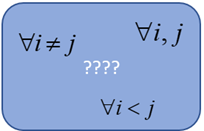
A standard problem in continuous time job-scheduling is to forbid jobs to overlap:

\[\begin{align}&S_i \ge E_j\\ &\text{or}\\ &S_j \ge E_i\end{align}\]

where \(S_i\) and \(E_i\) are start and finishing times of job \(i\):

In a MIP this is usually formulated as [1]:

\[\begin{align}&S_i\ge E_j - M\delta_{i,j}\\ &S_j \ge E_i - M(1-\delta_{i,j})\\ &\delta_{i,j} \in \{0,1\}\end{align}\]

Best choice: \(\forall i<j\)

If we compare job \(i\) with \(j\), we no longer need to check job \(j\) and \(i\). So often we implement the constraints only for the combinations \(i<j\) (of course \(\forall j>i\) would be just as valid).

In this post I want to investigate a bit what happens if we choose a different set of combinations over which we apply the constraints.

Case 2: \(\forall i,j\)

What happens if we are sloppy with this and compare for all \(i,j\)? If \(i=j\), we introduce an infeasibility that is easily detected by the solver. Some solvers do report:

Model is infeasible or unbounded

which is a little bit less helpful. In any case, the model will not solve if the modeler applies these constraints for all \(i,j\).

Case 3: \(\forall i\ne j\)

Now, what happens if we use \(\forall i\ne j\) instead of \(\forall i<j\)? This is actually something I see quite often in models (see [2] for an example). The solver (or modeling system) will not provide any feedback on this. It will solve the model and provides correct solutions in both cases.

What about solution times? There are two things to consider:

1. The number of binary variables \(\delta_{i,j}\) increases two-fold. However, implicitly the model enforces \(\delta_{i,j}=1-\delta_{j,i}\). If a variable \(\delta_{i,j}\) is fixed to zero or one, automatically \(\delta_{j,i}\) will also assume an integer value. The total impact of this on the node count of MIP solver is not clear to me. Indeed, the number of nodes is not uniformly better using either formulations.
2. The number of equations (and variables) involved increases by a factor of 2. This should slow down the LP relaxations solved by the MIP solvers. I would expect the speed in terms of the number of nodes per second or Simplex iterations per second to decrease. This turns out to be an important factor.

Let’s try this out on a smallish but difficult job shop problem [3].

Indeed we see no consistency in the node count. However the number of nodes per second and iterations per second behaved as I predicted. The total time is affected by this in such a manner that the funny difference in node count is not as significant as the difference in speed solving the LP relaxations. Even in cases where the node count or iteration count is better for the \(i\ne j\) model, it still loses out on total time. I.e. \(i<j\) is a winner, but may be for a different reason than you might think.

Conclusion: please use \(i<j\) when implementing the no-overlap equations.

References

1. Alan Manne, On the job-shop scheduling problem, Operations Research, Vol. 8, No. 2, March-April 1960.
2. ojAlgo Linear Optimization - Preventing work shift overlaps?, https://stackoverflow.com/questions/46823121/ojalgo-linear-optimization-preventing-work-shift-overlaps. I am not familiar with ojAlgo, but the presented model in the answer does seem to implement just \(i \ne j\).
3. Data set ft10 from H. Fisher, G. L. Thompson, Probabilistic learning combinations of local job-shop scheduling rules, in: J. F. Muth, G. L. Thompson (eds.),  Industrial Scheduling, Prentice Hall, Englewood Cliffs, N.J., 1963.