Word vs LaTeX

A software usability study comparing Word and LaTeX: http://journals.plos.org/plosone/article?id=10.1371/journal.pone.0115069. They claim Word is more productive. See also: http://www.nature.com/news/word-processing-war-flares-up-on-social-media-1.16669.

I will try to add a Word export facility to my GAMS documentation tool (http://yetanothermathprogrammingconsultant.blogspot.com/2014/12/convert-gams-to-latex.html) may be using MathType.

Scheduling as non-convex MIQP

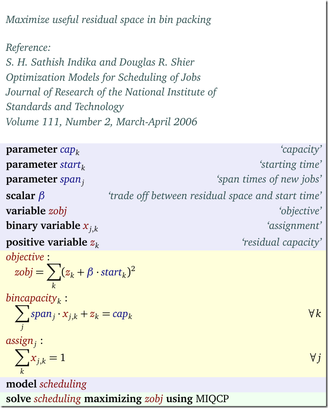
The following model tries to assign jobs to ‘bins’ (bins can be interpreted as workstations) in such a way that the remaining space in the bins is as large as possible (i.e. as little fragmentation as possible so that we have capacity left for large jobs). 

Essentially we place high value on large values on remaining capacity z_k. We consider here cases with β=0 (if β>0 we also like jobs to be executed early: remaining capacity more in the future is more valuable). This is a non-convex problem so not so easy to solve. This is also the model discussed here.

The choice of a quadratic objective is somewhat arbitrary. It is a simple function that has the required properties that larger values for z_k are valued more than proportionally (i.e. linear). In practice I often handle this by some piecewise linear formulation. In addition in practical cases it may be useful to give bins (workstations) without any jobs additional value (no set-up or clean-up in this case, so an unused bin may be preferred). 

With Cplex’s global MIQP solver (http://www.orsj.or.jp/ramp/2014/paper/4-3.pdf) we have now at least three ways to solve this problem with Cplex:(global MIQP, MIP with SOS2 interpolation, MIP with binaries exploiting integer data for capacity and job spans). Using an expanded (larger) version of the dataset provided in the paper with 27 bins and 15 jobs to allocate we try a few formulations.

• The global MIQP formulation uses the above model directly. We solve to optimality with 4 threads. Cplex selects this algorithm with option SolutionTarget=3.
• We can add a small value for β to try to reduce some symmetry in the model. We are still aiming for large remaining capacities, but we add a little bit of noise to distinguish similar solutions. The purpose is not really to add a ‘schedule as early as possible’ objective but rather just to increase the performance of the branch-and-bound algorithm. In the experiment we use β=0.01. Note: this may not always give us the same optimal solution.
• We can use a piecewise linear formulation using SOS2 variables. In this case we used 4 segments. Obviously this is an approximation, so we may arrive at a different optimal solution. However in this case just using 4 segments is good enough to find the global optimum.
• We can assume all capacity and job length data is integer (as is the case for the example data sets in the paper), and use this to formulate a linear model with extra binary variables. Essentially we implement a table lookup. If all data is integer valued (and the range of the numbers is not outrageously large) this will give us the proven optimal solution of the original MIQP. Exploiting properties of the input data can be key to solve things fast.

Here are the results:

These results confirm my experience. I typically use a piecewise linear formulation with just a few segments for this. In most cases I use even fewer than the 4 segments we used here. This seems often to perform reasonably well.

The authors of the original paper did not explore these alternatives but concluded quickly the global MIQP (implemented in Lingo) was too slow and implemented a heuristic. I am not sure if they would have done the same if they saw these results.

Update:

Instead of somewhat more complex formulations suggested in the comments, a simple table look-up using binary variables can be implemented with three constraints having a SOS1 structure:

This will make sure we have y=f(x) where x = 0,1,…,n. This is very close to the SOS2 formulation so took me just minutes to implement.

DropSolve

IBM has a cloud-based widget: just drop your input files and get a solution file back.

http://www-969.ibm.com/software/analytics/docloud/#demo

Stopping criteria for meta-heuristics

When running a really small non-convex MIQP problem with GAMS+Localsolver I see:

LocalSolver 5.0 (Win64, build 20141120) Copyright (C) 2014 Innovation 24, Aix-Marseille University, CNRS. All rights reserved (see Terms and Conditions for details). Searching for equations that define variables... found 5 Instance:       20 Variables                  9 Constraints                 82 Expressions                132 Operands     time |           iterations |         #infeas       0s |                    0 |               4     time |           iterations |       objective       1s |               583495 | 2.66000000e+002       2s |              1406684 | 2.66000000e+002       3s |              2235323 | 2.66000000e+002       4s |              3073170 | 2.66000000e+002       . . . . lots of lines with the same objective     998s |            677978972 | 2.66000000e+002     999s |            678600000 | 2.66000000e+002    1000s |            679218601 | 2.66000000e+002 Stopped due to time limit. Feasible solution found. Objective Value: 2.66000000e+002

Obviously the default stopping condition (max time = 1000s) is not very good for this case: we are just sitting there for 99.99% 99.9% of the time already at the optimal solution doing nothing useful. (266 is indeed the global optimum). In general these heuristics have no idea how close they are to an optimal solution, and just rely on the user to provide these time or iteration limits. (MIP solvers have this very powerful bounding information where we can say at any moment in time what the gap is between the best solution found an the best solution possible).

Is there nothing better we can do? There is some research on probabilistic stopping rules for these kind of algorithms (i.e. stop as soon as we think the probability we will find a better solution is small):

• Ribeiro, Rosseti, Souza, “Effective probabilistic stopping rules for randomized metaheuristics: GRASP implementations”, Learning and Intelligent Optimization, Lecture Notes in Computer Science Volume 6683, 2011, pp 146-160
• Boender, Rinnooy Kan, "Bayesian stopping rules for multistart global optimization methods", Mathematical Programming, 37:59–80, 1987.
• Dorea, "Stopping rules for a random optimization method", SIAM Journal on Control and Optimization, 28:841–850, 1990.
• Hart, "Sequential Stopping Rules for Random Optimization Methods with Applications to Multistart Local Search", SIAM Journal on Optimization, 1998, Vol. 9, No. 1 : pp. 270-290
• Safe, Carballido, Ponzoni, Brignole, “On Stopping Criteria for Genetic Algorithms”, Advances in Artificial Intelligence – SBIA 2004, Lecture Notes in Computer Science, 405-413, 2004

I would guess such a thing could well be a better default stopping rule.

PS Look at these iteration numbers. Don’t care here about a million iterations more or less. (Of course that is the whole purpose of this algorithm: do as many evaluations as possible).

Convert GAMS to LaTeX

Work in progress. This is automatically generated from compiled GAMS code. Part of a documentation tool to generate documentation for very large models. 

The different coloring of decision variables and parameters can help understanding the equations. In this case x is a parameter (this is typical when we implement estimation problems in GAMS: the statistical variables become parameters, while coefficients in the statistical model – here β and µ – are decision variables in the optimization model).

No multiple objectives?

In http://fdahms.com/2014/12/05/objective_functions/ it is argued that we should not fall in the “multi objective trap”. In my experience many practical models have some multi-objective structure. Some examples of models I have been working on are:

• Return vs risk. e.g. portfolio models
• Scheduling: minimize number of late (I should say tardy) jobs vs sum of of tardiness. If only number of late jobs is considered, it does not matter how late a late job is. In practice a job being late a little bit is better. On the other hand the minimizing the sum may deliver a ton of jobs being a little late. Combining these objectives can help.
• Scheduling: adding an extra objective that minimizes the difference between an existing schedule and the new schedule can help preventing wild changes in schedules without having a clear benefit (persistency).
• Cost vs Customer Service Level. If we can improve the CSL when it costs very little we may want to exploit this. On the other hand if a small decrease in CSL delivers a ton of profit then that is also worth considering.
• Tank design: cost vs fire power vs weight.
• Supply chain: cost vs robustness. E.g. keep extra suppliers although reducing the number of suppliers may reduce cost.
• In a typical  Cost – Benefit Analysis we also have to consider several criteria.
• Soft and elastic constraints will give rise to extra objectives.
• Etc, etc,

In my view many if not most interesting practical problems have conflicting goals and objectives. To make the client aware of this is an important role of a modeler. Even if we solve this as a single objective model using weights and penalties, the modeler needs to be aware and communicate the multi-objective nature and trade-offs of the underlying model.

Modeling number of machine start-ups

I came a across an extension of a well-known problem: counting the number of start-ups of a machine.

In the power generation models we often see constraints related to the number of start-ups of a generator: because of wear and tear we may like to minimize or restrict the number of times a generator is turned on. In the picture below the x(i) vector is the state of a generator (on or off) and the s(i) vector indicates when a startup occurs (i is time period). Both x and s are binary variables.

If we are minimizing the number of startups or have an upper bound, this can be easily modeled with a single inequality:

Here s(i) is forced to be one if there is a start-up, otherwise it is unrestricted. I.e. as long as the bound U is not binding we may have a few elements in s being 1 while there is no real start-up there. This is a structure we often see in models.

A lower bound on the number of startups is somewhat unusual, but lets see what happens. If we have a lower bound on the number of start-ups we need to be more precise and force s(i)=0 if there is no start-up. This can be modeled as:

This nonlinear expression can be linearized easily and leads to the three inequalities shown above. This formulation is so tight we can even relax the s variables to continuous variables between zero and one (they will be automatically integer for any feasible solution).

The state in period zero is assumed to be known. This matters if we have x(i)=1 in the first period. This is only counted as a startup in case the initial state is 0. In GAMS we can model this compactly as:

The trick with the initial state resembles how we can deal with iniitial inventory in a supply chain model. See: http://yetanothermathprogrammingconsultant.blogspot.com/2014/10/handling-of-inventory.html.

Gurobi 6 Distributed vs Concurrent MIP

The new Gurobi 6 has quite an attractive offering for running distributed MIPs. Here is a summary for their results (MIPLIB models taking more than 100s).

The concurrent MIP method is just running the same model on different machines with a different random number seed. This changes the solution path sufficiently to actually form a feasible parallel approach. The solution time is the time of the winner. This method always amazes me, but also makes me feel somewhat uncomfortable (the scary question is: if this scheme works does the MIP solver really know what it is doing? – My answer often depends on whether the last MIP I tried was solved ok.). See e.g.: http://coral.ie.lehigh.edu/~jeff/mip-2008/talks/danna.pdf

The distributed MIP is really a distributed MIP where each machine works on parts of the tree. Happy to see this actually works a bit better. Before you buy a ton of machines note that performance starts to tail off after using more than 8 machines. Some numbers showed that a bunch of smaller machines may show better performance than a huge multi-core machine (these SMP machine suffer from memory contention, probably exacerbated by MIP solvers jumping around in memory i.e. suffering from limited locality which hampers exploiting even large caches). Typically several small machines is cheaper than one big one.

Note that every machine in the above picture is actually equipped with a 4 core CPU, so we already have significant parallelism on each machine.

Some other new features:

• Some support for piecewise linear functions. In the objective only and convex only so for a limited class of models for now. Non-convex functions are translated into a MIP formulation.
• General improvements in performance
• Enhancements in lazy constraints

Optimization in R

Some interesting notes:

From: http://user2014.stat.ucla.edu/files/tutorial_Nash_slides.pdf:

My opinion: I think GAMS and R non-linear optimization really targets different audiences and different model types (R: smaller models with emphasis on parameter estimation and zero or few constraints; GAMS: large, sparse and more complex models with many constraints). Matlab and R may be seen a little bit more as direct “competitors” with respect to the type models they typically solve.

Amazon seems to confirm people are using R to do optimization:

Big Iron vs my laptop

In this post a question is being asked about MIP solvers running on a cluster. In my answer I note that I usually prefer to be able to run models comfortably on my laptop (it is somewhat souped up with e.g. 32 gb RAM). When comparing running models on your own machine vs a compute cluster we can distinguish four cases:

1. Model runs runs fast on both. This is what I like most. In this case of course running locally is often easier: the big iron does not really help. This is a large class of problems (helped by good solvers and lots of modeling experience). 
2. Model runs slow on laptop and slow on big machine. The expensive hardware does not help here. This also happens quite frequently. Solution: rework the problem (e.g. reformulations, aiming for good solutions, heuristics etc). Hopefully moving the problem to category 1.
3. Model runs slow on my laptop but fast on the big machine. This actually does not happen too often. The number of models that falls in this category is surprisingly small.
4. Model runs fast on my laptop and slow on the big machine. This should not happen, but it actually does. Often my optimization problems run surprisingly slow on expensive hardware. Some reasons: the cluster has expensive hardware from a few years ago (my laptop is new every year), there may be latencies in starting jobs on a cluster, it may have been too expensive to get the best solvers on the big machines (I think IBM counts VPUs which can add up) or much parallelization does not pay off. Big caches may help less than expected for some sparse data structures used in modeling systems and solvers. Another reason is often; not enough memory. Running n parallel jobs may require n times the memory. I have seen clients being somewhat underwhelmed or even disappointed by performance on what was sold as very expensive (and fast) hardware. 

Sometimes big hardware can help when evaluating many scenarios or if different users want to solve things at the same time (e.g. some web service).