Solving DEA Models with GAMS

Data Envelopment Analysis (DEA) models are somewhat special. They typically consist of small LPs, of which a whole bunch have to be solved. The CCR formulation (after [1]), for the \(i\)-th DMU (Decision Making Unit), can be stated as [2]:

CCR LP Model

\[\begin{align} \max \>& \color{darkred}{\mathit{efficiency}}_i=\sum_{\mathit{outp}} \color{darkred}u_{{\mathit{outp}}} \cdot \color{darkblue}y_{i,{\mathit{outp}}} \\ & \sum_{\mathit{inp}} \color{darkred}v_{{\mathit{inp}}} \cdot \color{darkblue}x_{i,{\mathit{inp}}} = 1 \\ & \sum_{\mathit{outp}} \color{darkred}u_{{\mathit{outp}}} \cdot \color{darkblue}y_{j,{\mathit{outp}}} \le \color{darkred}v_{{\mathit{inp}}} \cdot \color{darkblue}x_{j,{\mathit{inp}}} && \forall j \\ & \color{darkred}u_{{\mathit{outp}}} \ge 0, \color{darkred}v_{{\mathit{inp}}} \ge 0 \end{align}\]

Like we see in statistical models, \(\color{darkblue}x\) and \(\color{darkblue}y\) are data. The weights \(\color{darkred}u\) and \(\color{darkred}v\) are decision variables.

We have a solve loop here. GAMS solve loops are slow. For many cases, this is not a very big deal as the solution time spent inside the solver will dominate the total turnaround time. For these DEA-type models, however, we have very small LPs to be solved inside the loop. Suddenly, the overhead is very large. What can we do? Here are some remedies:

1. GAMS options. GAMS prints a lot of information to the listing file. This is great for debugging, but it is a bit much when we are dealing with a solve loop. We can turn off all this printing. Another option is to call a solver DLL instead of an EXE. Calling an EXE gives some advantages, but in this case, it has a non-trivial overhead. A further detail is that by default, GAMS will save all its data before a solve, so the solver can use all the available memory. When GAMS restarts after a solve, it needs first to read this data. With a DLL interface, this is not done: GAMS stays in memory while the solver is running. The two options we are talking about are solprint and solvelink, and they can be changed easily. 
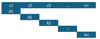
2. Solve as one big model. Instead of solving many tiny models, we can combine them into one big model. This will have a block-diagonal structure. 
   
   
   
   This is always a nice modeling exercise (adding an index — a concept that is not always obvious to students). In theory, solving a series of smaller LPs is better than solving one big one (as LP algorithms do not have linear run-time). In practice, things are different. This demonstrates the limited value of complexity theory when working with a given model on a given data set (another important lesson for students).
3. Use the GAMS scenario solver [3]. This essentially performs the loop inside the solver (or, more precisely, close to the solver) instead of inside GAMS. 

Using a random data set with \(n=500\) DMUs, 5 inputs, and 5 outputs, we get the following results:

Version	Description	Total Time (seconds)
1	Standard GAMS Loop	18
2	Options Solprint=silent,Solvelink=5	6
3	Single block-diagonal model	3
4	Scenario solver	1

One way of interpreting these results is: using a standard GAMS loop, the total turnaround time is 18 seconds, of which 17 seconds is overhead.

Sorting in GAMS

The sorting step shown at the end of the GAMS code is also worth studying. Sorting is an interesting concept in GAMS. Suppose we observe efficiencies as follows:

----    116 PARAMETER efficiency  efficiency of each DMU

DMU1  0.803,    DMU2  0.540,    DMU3  0.362,    DMU4  1.000,    DMU5  0.569,    DMU6  0.651,    DMU7  1.000,    DMU8  0.119
DMU9  0.428,    DMU10 1.000

We can calculate a ranking by:

    rank(i) = sum(ii$(efficiency(ii)>=efficiency(i)), 1);

This yields:

----    137 PARAMETER rank  number of DMUs with better or equal efficiency

DMU1   4.000,    DMU2   7.000,    DMU3   9.000,    DMU4   3.000,    DMU5   6.000,    DMU6   5.000,    DMU7   3.000
DMU8  10.000,    DMU9   8.000,    DMU10  3.000

Next, create an extra index, indicating the rank:

  parameter ranked_eff(r,i) 'ranked efficiency';

  ranked_eff(r,i)=efficiency(i)$(rank(i)=ord(r));

The result is a sorted parameter:

----    142 PARAMETER ranked_eff  ranked efficiency

rnk3 .DMU4  1.0000,    rnk3 .DMU7  1.0000,    rnk3 .DMU10 1.0000,    rnk4 .DMU1  0.8031
rnk5 .DMU6  0.6515,    rnk6 .DMU5  0.5693,    rnk7 .DMU2  0.5399,    rnk8 .DMU9  0.4285
rnk9 .DMU3  0.3617,    rnk10.DMU8  0.1189

If efficiencies are identical, they get the same rank.

Conclusion

We face a longish solve loop with very small but independent LPs. This particular structure provides some opportunities to achieve significantly better performance.

The solution is easier to interpret when we sort things. A good opportunity to show how this can be done in GAMS.

References

1. A. Charnes, W. W. Cooper, E. Rhodes, Measuring the efficiency of decision-making units. European Journal of Operational Research, 1978, 2, pp. 429-444.
2. Tutorial model from https://www.deazone.com/
3. https://www.gams.com/modlib/adddocs/gusspaper.pdf

Appendix: GAMS model

Implementation of all four methods:

1. Default GAMS loop. Use a singleton set to hold the current DMU.
2. As 1, but using GAMS options solprint and solvelink to speed things up.
3. One large block-diagonal model formed by adding an index to the weight variables \(\color{darkred}u\) and \(\color{darkred}v\).
4. Using the scenario solver.

Notice the sorting step at the end to make the results more meaningful.

$ontext      Data Envelopment Analysis (DEA) Performance       Different GAMS formulations       Reference:       A. Charnes, W. W. Cooper, E. Rhodes,       Measuring the efficiency of decision making units.       European Journal of Operational Research 1978, 2, 429-444         www.deazone.com          This is to explore some different GAMS formulations     for these kinds of models.        version                             total time       1   default loop                    18       2   solprint=silent, solvelink=5     6       3   solve as one big model           3       4   use scenario solver              1     $offText   *---------------------------------------------------------------- * select version to run *----------------------------------------------------------------   $set version 1 * 1 : default loop model * 2 : reduce output to listing file and use solver DLL * 3 : solve as one big model * 4 : solve using the scenario solver   *---------------------------------------------------------------- * random data *----------------------------------------------------------------    sets i       "DMU's"  /DMU1*DMU500/      j       'inputs and outputs' /in1*in5,out1*out5/      inp(j)  'inputs'  /in1*in5/      outp(j) 'outputs' /out1*out5/ ;   alias (i,ii,dmu);   parameter data(i,j) 'random data set'; data(i,j) = uniform(1,100); display data;   * like in statistical models, x,y are data in this * formulation parameter    x(i,inp)  'inputs of DMU i'    y(i,outp) 'outputs of DMU i' ; x(i,inp) = data(i,inp); y(i,outp) = data(i,outp);   parameter efficiency(i) 'efficiency of each DMU';   *---------------------------------------------------------------- * loop version *----------------------------------------------------------------   $if %version%==1 $set doloop 1 $if %version%==2 $set doloop 1   $ifthen %doloop%==1   *---------------------------------------------------------------- * Standard CCR model *----------------------------------------------------------------   singleton set i0(i) 'current DMU (assigned inside solve loop)';   positive variables    v(inp)  'input weights'    u(outp) 'output weights' ;   variable    eff 'efficiency' ;   equations    objective  'objective function: maximize efficiency'    normalize  'normalize input weights'    limit(i)   "limit other DMU's efficiency";   objective..  eff =e= sum(outp, u(outp)*y(i0,outp)); normalize..  sum(inp, v(inp)*x(i0,inp)) =e= 1; limit(i)..   sum(outp, u(outp)*y(i,outp)) =l= sum(inp, v(inp)*x(i,inp));   model dea /objective, normalize, limit/;   *---------------------------------------------------------------- * Solve loop *----------------------------------------------------------------   * optional options *  solprint=silent : reduce amount of information written to the listing files *  solvelink=%solveLink.loadLibrary% : use solver DLLs   $if %version%==2 option solprint=silent, solvelink=%solveLink.loadLibrary%;   loop(dmu,   * current DMU in model    i0(dmu) = yes;    * solve LP    solve dea using lp maximizing eff;    abort$(dea.modelstat<>1) "LP model 'dea' was not optimal";   * collect result    efficiency(dmu) = eff.l; ); display efficiency;   $endif   *---------------------------------------------------------------- * Combined block-diagonal CCR model * just one solve *----------------------------------------------------------------   $ifthen %version%==3   option solprint=silent, solvelink=%solveLink.loadLibrary%;   positive variables    v(inp,i)   'input weights'    u(outp,i)  'output weights' ;   variable    eff(i)      'efficiency of each DMU'    totaleff    'summation of all efficiencies' ;   equations    objective(i)   'objective function: maximize efficiency'    normalize(i)   'normalize input weights'    limit(i,ii)    "limit other DMU's efficiency"    totalobj       'combines all individual objective functions' ;   totalobj..       totaleff =e= sum(i, eff(i)); objective(i)..   eff(i) =e=  sum(outp, u(outp,i)*y(i,outp)); normalize(i)..   sum(inp, v(inp,i)*x(i,inp)) =e= 1; limit(i,ii)..    sum(outp, u(outp,ii)*y(i,outp)) =l= sum(inp, v(inp,ii)*x(i,inp));   model dea2 /objective, normalize, limit, totalobj/; solve dea2 using lp maximizing totaleff; abort$(dea2.modelstat<>1) "LP model 'dea2' was not optimal";   efficiency(i) = eff.l(i);   $endif   *---------------------------------------------------------------- * Using the scenario solver * just one solve statement * loop is done inside solver * model is almost the same as under versions 1 and 2 *----------------------------------------------------------------   $ifthen %version%==4   parameter   y0(outp)   x0(inp) ;   positive variables    v(inp)  'input weights'    u(outp) 'output weights' ;   variable    eff 'efficiency' ;   equations    objective   'objective function: maximize efficiency'    normalize   'normalize input weights'    limit(i)    "limit other DMU's efficiency";   objective..  eff =e= sum(outp, u(outp)*y0(outp)); normalize..  sum(inp, v(inp)*x0(inp)) =e= 1; limit(i)..   sum(outp, u(outp)*y(i,outp)) =l= sum(inp, v(inp)*x(i,inp));   model dea /objective, normalize, limit/;   set headers report / modelstat, solvestat, objval /; parameter     scenrep(i,headers) 'solution report summary'     scopt / SkipBaseCase 1 /;   set dict / i      .scenario.''            x0     .param.   x            y0     .param.   y            eff    .level.   efficiency            scopt  .opt.     scenrep /;   x0(inp) = 0; y0(outp) = 0; solve dea using lp max eff scenario dict; display scenrep,efficiency;   abort$sum(i$(scenrep(i,'modelstat')<>1),1) "Not all LPs were optimal";   $endif   *---------------------------------------------------------------- * create sorted output *---------------------------------------------------------------- set r /rnk1*rnk1000/;   parameter rank(i) 'number of DMUs with better or equal efficiency'; rank(i) = sum(ii$(efficiency(ii)>=efficiency(i)), 1); display rank;   parameter ranked_eff(r,i) 'ranked efficiency'; ranked_eff(r,i)=efficiency(i)$(rank(i)=ord(r)); option ranked_eff:4:0:4; display ranked_eff;