GAMS + R scripting

 I like to automate things. That means in practice: I write scripts. I prefer to spend a little more time to develop a script, basically for two reasons:

• A script can be executed again with little or no effort.
• A script serves as documentation. 

This helps to make things reproducible.

Here is a setup I often use for post-processing GAMS results with R. 

$ontext    Generate data in GAMS and plot in R. $offtext *--------------------------------------------------- * generate some random data points *--------------------------------------------------- set    i 'points' /p1*p70/    c 'coordinates' /x,y/ ; parameter p(i,c) 'points'; p(i,c) = uniform(0,100); display p; *--------------------------------------------------- * make plot *--------------------------------------------------- * GAMS macros $set script     script.R $set gdx        data.gdx $set pdf        plot.pdf $set title      data points $set rcommand   '"c:\Program Files\R\R-4.0.3\bin\Rscript.exe" --vanilla %script%' * create gdx file with data execute_unload "%gdx%",p; * run the R script execute '%rcommand%'; * launch a pdf viewer to show the result execute 'shellexecute %pdf%'; *--------------------------------------------------- * R script *--------------------------------------------------- $onecho > %script% options(echo=TRUE) library(gdxrrw)      # for reading GDX files library(tidyverse)   # for plotting and pivoting # read parameter p from GDX file p <- rgdx.param("%gdx%","p") head(p) # convert from long to wide format. x,y as columns. p2 <- pivot_wider(p,id_cols=i,names_from=c,values_from=p) head(p2) ggplot(p2, aes(x=x,y=y)) + geom_point() + ggtitle("%title%") ggsave("%pdf%") $offecho

The first step is here: generate some data in GAMS. For this case, we have 70 random 2-d data points. If we look at the display output (first 10 points), we see:

 

----     18 PARAMETER p  points

              x           y

p1       17.175      84.327
p2       55.038      30.114
p3       29.221      22.405
p4       34.983      85.627
p5        6.711      50.021
p6       99.812      57.873
p7       99.113      76.225
p8       13.069      63.972
p9       15.952      25.008
p10      66.893      43.536

That this is shown with two data columns is just representation. When shown in list- or long-format, we see:

----     19 PARAMETER p  points

p1 .x 17.175
p1 .y 84.327
p2 .x 55.038
p2 .y 30.114
p3 .x 29.221
p3 .y 22.405
p4 .x 34.983
p4 .y 85.627

The parameter p is exported to a gdx file (a binary GAMS data file).

The next step is to use an R script that has to read the GAMS data and make a simple plot. To make the GAMS file self-contained, we just make the script part of the GAMS model and echo it to a file script.R. I typically put this at the bottom of my GAMS script. Just for aesthetical reasons: I prefer this big piece of R code not to be in the middle of my GAMS code. At the bottom, it is just a bit out of the way. The reason we can do this, is that GAMS is a two-pass system: compilation followed by execution. The $echo command is compile-time so we can put this at the bottom of the file: it will be echoed before we start executing GAMS commands like execute '%rcommand%'; 

Some file names are used multiple times. I also may want to high-lite some names a bit, so they are not being buried somewhere in the middle of some code. I often prefer to collect these names in a collection of GAMS macros. This is like a #define in some programming languages. Similar to MS-DOS batch files, we use $set to define a name and %name% to reference a name. An advantage of using $echo is that we can reference these defined names in the R script. An occurrence of %name% will be substituted out for the defined name before the script is echoed to the file. 

Let's go through the R script a bit.

When we run the script, it is often useful to echo the commands before they are executed. If something goes wrong, you will know exactly in what command this happened. In addition, if the script takes a bit of time to run, you have some indication of where we are. This is the reason I added options(echo=TRUE) as the first line of the script.

The R script needs to read the GAMS data that is stored in the gdx file. We do this here with the R package gdxrrw (is part of the GAMS distribution or can be downloaded from the GAMS web site -- the version in the GAMS distribution is rather outdated, so I suggest to download it).  The other package I use here is tidyverse. It contains the ggplot plotting package and we also use the pivot_wider command from this package. 

So we start with reading the GAMS data. The data arrives as a data frame. The head command is used to show a few records, so we can see the structure. The log shows:

> # read parameter p from GDX file

> p <- rgdx.param("data.gdx","p")

> head(p)

   i c        p

1 p1 x 17.17471

2 p1 y 84.32667

3 p2 x 55.03754

4 p2 y 30.11379

5 p3 x 29.22121

6 p3 y 22.40529

I.e. the data arrives in "long format". For the benefit of ggplot, we want x and y to be columns. In R this is not just a question of representation: we physically have to apply a pivot operation. We use the command  pivot_wider for this. The results look like:

> # convert from long to wide format. x,y as columns.

> p2 <- pivot_wider(p,id_cols=i,names_from=c,values_from=p)

> head(p2)

# A tibble: 6 x 3

  i         x     y

  <fct> <dbl> <dbl>

1 p1    17.2   84.3

2 p2    55.0   30.1

3 p3    29.2   22.4

4 p4    35.0   85.6

5 p5     6.71  50.0

6 p6    99.8   57.9

The head(p2) command prints the result in a slightly different way. First, p2 is not strictly a data frame but rather a tibble. Essentially this is a data frame plus some extra facilities. More importantly, we indeed see that we now have the data in "wide format" with x and y as columns. Conversions between wide and long format data are quite common, so it is good to know about this.

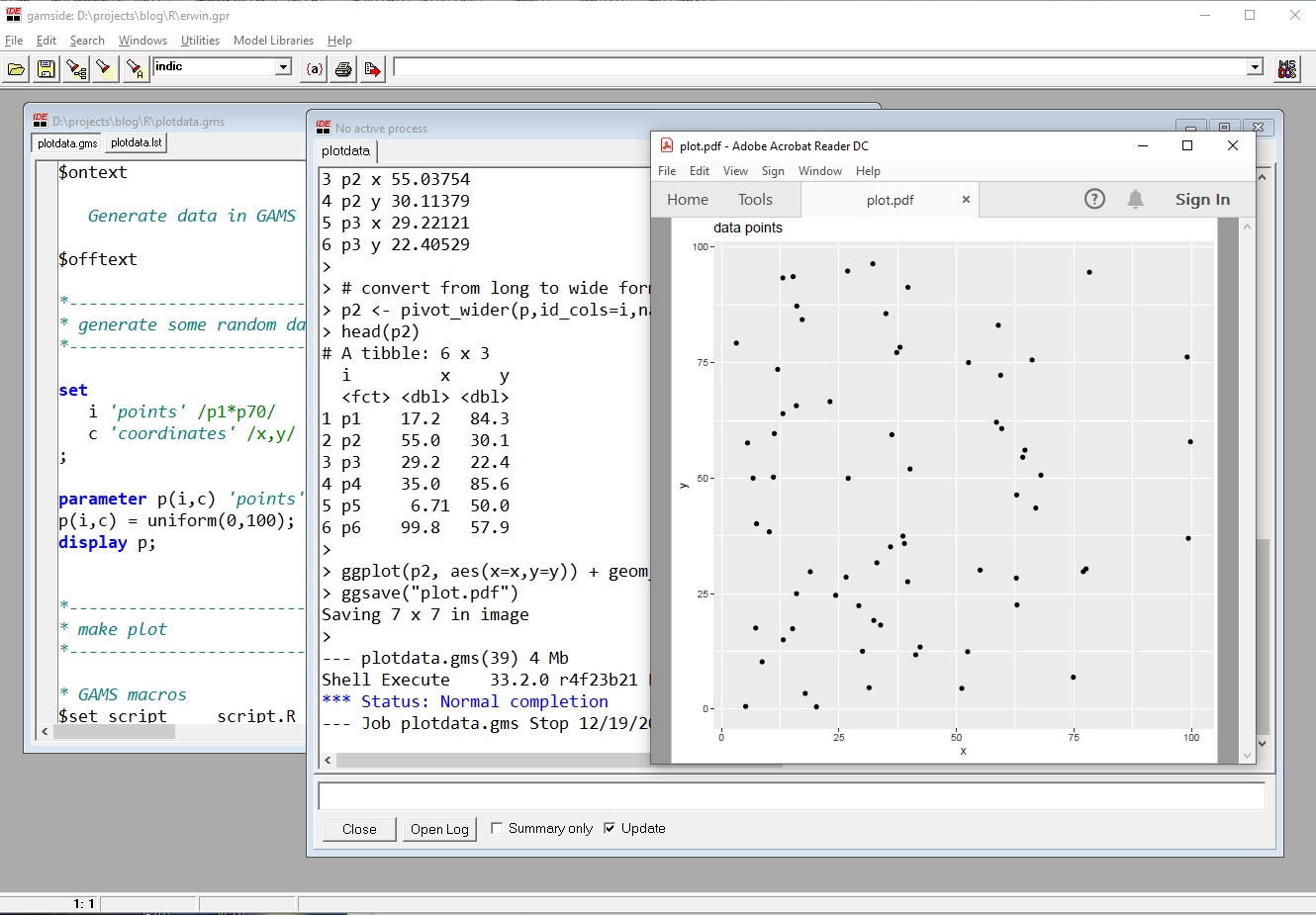
Now we are ready to plot. We use no-frills ggplot to produce an x-y scatter plot. Finally, the results are saved to a PDF file.  

The GAMS code will show the PDF file, so you will see something like:

Notes:

• This is a simple example, but this is a scheme I often use, even for more complex things.
• I often develop the R script in Rstudio, and then copy a working version into a GAMS script. 
• Alternatives to gdxrrw include using CSV files or gdx2r.exe (this converts a GDX file into an .Rdata file).
• R code can be difficult to read. I tend to add a lot of comments to my code.
• GAMS data is stored sparse, so zeros are not stored and not exported to R. This can trip you up. In this example: a point (0,0) would not be in the GDX file.
• Interfaces between different programs can be a bit difficult to understand and develop. In this case: you need to know GAMS and you need to know R. In addition, these two programs have different views of the world. GAMS works with sparse multi-dimensional parameters, indexed by sets (strings) and R works with data frames. There can be surprises when we want to cross from one paradigm to another.