A pure fixed charge transportation problem

The standard transportation problem is an example of an easy linear programming problem:

Transportation Problem
\[\begin{align}\min & \sum_{i,j} \color{DarkBlue} c_{i,j} \color{DarkRed} x_{i,j}\\ & \sum_j \color{DarkRed} x_{i,j} = \color{DarkBlue} {\mathit{supply}}_i\\ & \sum_i \color{DarkRed} x_{i,j} = \color{DarkBlue} {\mathit{demand}}_j \\ & \color{DarkRed} x_{i,j} \ge 0\end{align}\]

We can solve very large instances very quickly. The fixed charge transportation problem is much more difficult:

Fixed Charge Transportation Problem

\[\begin{align}\min & \sum_{i,j} \color{DarkBlue} c_{i,j} \color{DarkRed} x_{i,j} + \color{DarkBlue} d_{i,j} \color{DarkRed} y_{i,j}\\ & \sum_j \color{DarkRed} x_{i,j} = \color{DarkBlue} {\mathit{supply}}_i\\ & \sum_i \color{DarkRed} x_{i,j} = \color{DarkBlue}{\mathit{demand}}_j \\ & 0 \le \color{DarkRed} x_{i,j} \le \color{DarkBlue} M \color{DarkRed} y_{i,j}\\ & \color{DarkRed} y_{i,j} \in \{0,1\}\end{align}\]

Here we have an additional cost \(d_{i,j}\) if link \(x_{i,j}\) is used (i.e. if \(x_{i,j}\gt 0\)).  The binary variable \(y_{i,j}\) indicates if link \(i \rightarrow j\) is used. I.e. we want: \[y_{i,j} = 0 \Rightarrow x_{i,j}=0\] The constraint \(x_{i,j} \le M y_{i,j}\) is a big-M formulation for this. Notice that we do not need to worry about \(x_{i,j}=0 \Rightarrow y_{i,j}=0\): this will be taken care of automatically (because of the objective function). In practice we can do \[\begin{align} & x_{i,j} \le M_{i,j} y_{i,j}\\ & M_{i,j} = \min \{ \mathit{supply}_i,  \mathit{demand}_j \}\end{align}\] This gives some reasonable values for \(M_{i,j}\). A problem with only fixed charge costs (i.e. \(c_{i,j}=0\)) is sometimes called a pure fixed charge transportation problem. If we just want to minimize the number of links that are being used we can set \(c_{i,j}=0\) and \(d_{i,j}=1\). These models can be incredibly difficult to solve to proven optimality.

Here we try to solve a very small problem with 10 source nodes and 10 destination nodes. I used random values for the supply and demand:

----     20 PARAMETER supply  

src1  0.041,    src2  0.203,    src3  0.132,    src4  0.072,    src5  0.070,    src6  0.054,    src7  0.084
src8  0.206,    src9  0.016,    src10 0.120


----     20 PARAMETER demand  

dest1  0.178,    dest2  0.103,    dest3  0.177,    dest4  0.136,    dest5  0.023,    dest6  0.114,    dest7  0.028
dest8  0.045,    dest9  0.119,    dest10 0.078

The objective is \(\min \sum_{i,j} y_{i,j}\), i.e. we minimize the number of open links. This means we have just 100 binary variables. After setting a time limit of 9999 seconds I see:

. . .  5938307 5589691       15.7946    12       18.0000       15.0950 1.71e+08   16.14%  5946634 5596825       15.1040    25       18.0000       15.0950 1.72e+08   16.14%  5959435 5611506       15.1737    19       18.0000       15.0950 1.72e+08   16.14% Elapsed time = 9977.59 sec. (3226694.74 ticks, tree = 38155.78 MB, solutions = 3) Nodefile size = 36108.12 MB (23960.92 MB after compression)  5965049 5616397       16.0000    19       18.0000       15.0950 1.72e+08   16.14% Cover cuts applied:  264 Flow cuts applied:  5 Mixed integer rounding cuts applied:  331 Zero-half cuts applied:  4 Multi commodity flow cuts applied:  4 Root node processing (before b&c):   Real time             =    0.88 sec. (41.53 ticks) Parallel b&c, 8 threads:   Real time             = 10021.94 sec. (3248441.83 ticks)   Sync time (average)   = 5484.02 sec.   Wait time (average)   =    0.11 sec.                           ------------ Total (root+branch&cut) = 10022.81 sec. (3248483.36 ticks) MIP status(107): time limit exceeded Cplex Time: 10023.03sec (det. 3248483.36 ticks)

Ouch.. If you would have asked before, I certainly would have predicted somewhat better performance.

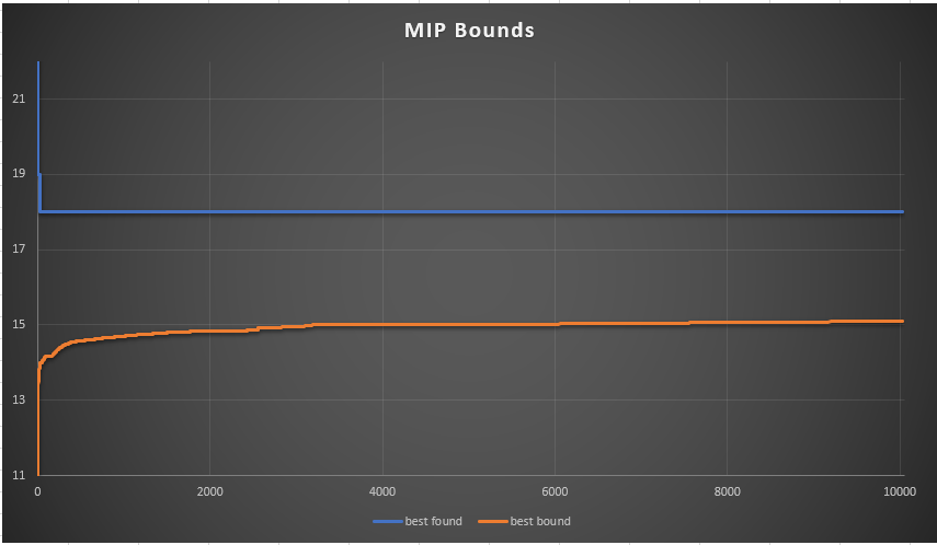MIP bounds don't change anymore

The best objective value of 18 was found after 25 seconds.  We might as well have stopped at that point...

Most likely 18 is the optimal objective, but we have not proven that. The best solution looks like:

Best found solution