Problem
We have \(N\) jobs to schedule. Each job has a given processing time. In addition we have a setup time for the machine in between jobs. The twist is that the required setup time depends on how two consecutive jobs differ. If two jobs in a row are very similar, the intermediate setup time is small, while if they are very different, the setup time increases. An example of such a problem is running some kind of printing jobs. Changing from a black job to a white job requires extensive cleaning, while white followed by black does not require much cleaning at all. See e.g. [1].
Some extra things to think about:
- The last job performed (called initial below) may be important, as we may need to do a setup from the initial state to whatever the selected first job is.
- The setup times are organized as an \((N+1) \times N\) matrix (one extra row for the initial job).
- We can have due dates and release dates on the jobs. We need to finish a job before the due date and cannot start a job before its release date.
- We may have some precedence relations: some jobs must be finished before another.
- We want to sequence the jobs such that the completion time of the last job is minimized (of course subject to due date, release date and precedence constraints).
Example data
Some random data can help to understand the problem a bit better.
----     26 PARAMETER proctime  processing time

job1  2.546,    job2  8.589,    job3  5.953,    job4  3.710,    job5  3.630,    job6  3.016,    job7  4.148
job8  8.706,    job9  1.604,    job10 5.502,    job11 9.983,    job12 6.209,    job13 9.920,    job14 7.860
job15 2.176


----     26 PARAMETER setup  setup time

               job1        job2        job3        job4        job5        job6        job7        job8        job9

initial       3.559       1.638       2.000       3.676       2.741       2.439       2.406       1.526       1.600
job1                      3.010       1.641       4.490       2.060       2.143       3.376       3.891       3.513
job2          1.728                   3.243       4.080       2.191       3.644       4.023       3.510       2.135
job3          1.291       1.703                   4.001       1.712       1.137       3.341       3.485       2.557
job4          4.134       2.200       1.502                   1.277       1.808       1.020       2.078       2.999
job5          4.974       2.480       2.492       4.088                   4.652       1.478       3.942       1.222
job6          1.903       2.584       2.104       1.609       4.745                   1.539       2.544       2.499
job7          1.407       2.536       2.296       1.769       1.449       3.386                   1.180       4.132
job8          3.026       1.637       3.628       3.096       1.498       4.947       1.912                   4.107
job9          3.940       1.342       1.601       2.737       1.748       3.771       4.052       1.619
job10         1.348       3.162       1.507       3.936       1.453       2.953       4.182       2.968       3.134
job11         1.099       1.711       1.245       1.067       4.343       3.407       1.108       1.784       4.803
job12         2.573       4.222       3.164       2.563       3.231       4.731       2.395       1.033       4.795
job13         3.321       1.666       3.573       2.377       4.649       4.600       1.065       2.475       3.658
job14         2.986       1.180       4.095       3.132       3.987       3.880       3.526       1.460       4.885
job15         4.163       3.441       1.217       2.941       1.210       3.794       1.779       1.904       4.255

      +       job10       job11       job12       job13       job14       job15

initial       3.356       4.324       1.923       3.663       4.103       2.215
job1          2.855       2.653       1.471       2.257       1.186       2.354
job2          1.346       1.410       3.565       3.181       1.126       4.169
job3          2.435       1.972       1.986       1.522       4.734       2.520
job4          1.605       1.697       2.323       2.268       2.288       4.856
job5          3.305       1.206       1.024       2.605       3.080       3.516
job6          2.074       4.793       1.756       2.190       1.298       2.605
job7          4.783       3.386       3.429       2.450       3.376       3.719
job8          4.730       1.805       2.189       1.789       1.985       3.586
job9          3.782       4.383       3.451       4.904       1.108       1.750
job10                     3.175       2.805       4.901       1.735       1.654
job11         2.342                   2.037       3.563       1.621       2.840
job12         3.288       2.335                   4.066       1.440       4.979
job13         3.374       1.138       4.367                   3.032       2.198
job14         3.827       4.945       4.419       3.486                   3.804
job15         4.967       4.003       3.873       1.002       2.055


----     26 PARAMETER due  due date

job3  28.569,    job5  98.104,    job6  27.644,    job7  55.274,    job8  57.364,    job11 60.875,    job12 96.637
job13 77.888


----     26 PARAMETER release  release time

job5  19.380,    job8  48.657,    job10 27.932,    job13 24.876


----     26 SET prec  precedence restrictions

            job3

job1         YES
job2         YES
Some jobs have release and due dates. The precedence restrictions say we need to do job 1 and 2 before job 3. The setup times are displayed as a matrix: \(\mathit{setup}_{i,j}\) is the setup time between jobs \(i\) and \(j\). Notice the extra row "initial" which is the last job from the previous planning period. The diagonal elements \(\mathit{setup}_{i,i}\) are not used.
Model
To model this, I use five sets of variables:
| Variable | Description |
|---|---|
| \(\color{DarkRed}{\mathit{First}}_j \in \{0,1\}\) | indicates the first job |
| \(\color{DarkRed}{\mathit{Last}}_j \in \{0,1\}\) | the last job |
| \(\color{DarkRed}{X}_{i,j} \in \{0,1\}\) | job \(j\) immediately follows job \(i\) |
| \(\color{DarkRed}{\mathit{StartTime}}_j \ge 0\) | the start time (after setup) of job \(j\) |
| \(\color{DarkRed}{\mathit{LastTime}}\) | Objective variable: completion time of last job |
The idea is that a job sequence \(1-2-3\) is encoded as:
- \(\color{DarkRed}{\mathit{First}}_1=1\)
- \(\color{DarkRed}{X}_{1,2}=\color{DarkRed}{X}_{2,3}=1\)
- \(\color{DarkRed}{\mathit{Last}}_3=1\)
The model itself looks like:
| No | Equation | Description |
|---|---|---|
| 1 | \[\min \color{DarkRed}{\mathit{LastTime}}\] | objective |
| 2 | \[\sum_j \color{DarkRed}{\mathit{First}}_j = 1\] | exactly one first job |
| 3 | \[\sum_j \color{DarkRed}{\mathit{Last}}_j = 1\] | exactly one last job |
| 4 | \[\color{DarkRed}{\mathit{Last}}_i+\sum_{j\ne i} \color{DarkRed}{X}_{i,j} = 1\>\>\forall i\] | job \(i\) is the last job or it has a successor \(j\) |
| 5 | \[\color{DarkRed}{\mathit{First}}_j+\sum_{i\ne j} \color{DarkRed}{X}_{i,j} = 1\>\>\forall j\] | job \(j\) is the first job or it has a predecessor \(i\) |
| 6 | \[\color{DarkRed}{\mathit{StartTime}}_j \ge \color{DarkBlue}{\mathit{setup}}_{\text{initial},j} \color{DarkRed}{\mathit{First}}_j \>\>\forall j\] | calculate start time of first job |
| 7 | \[\color{DarkRed}{\mathit{StartTime}}_j \ge \color{DarkRed}{\mathit{StartTime}}_i + \color{DarkBlue}{\mathit{proctime}}_i + \color{DarkBlue}{\mathit{setup}}_{i,j} - M(1-\color{DarkRed}{X}_{i,j})\>\>\forall i\ne j\] | calculate start time of job \(j\) with predecessor \(i\) |
| 8 | \[\color{DarkRed}{\mathit{LastTime}} \ge \color{DarkRed}{\mathit{StartTime}}_j + \color{DarkBlue}{\mathit{proctime}}_j\>\>\forall j\] | calculate completion time of last job |
| 9 | \[\color{DarkRed}{\mathit{StartTime}}_j \ge \color{DarkBlue}{\mathit{release}}_j \>\>\forall j \] | lower bound on start time |
| 10 | \[\color{DarkRed}{\mathit{StartTime}}_j \le \color{DarkBlue}{\mathit{due}}_j - \color{DarkBlue}{\mathit{proctime}}_j \>\>\forall j|\color{DarkBlue}{\mathit{due}}_j>0 \] | upper bound on start time |
| 11 | \[ \color{DarkRed}{\mathit{StartTime}}_j \ge \color{DarkRed}{\mathit{StartTime}}_i + \color{DarkBlue}{\mathit{proctime}}_i \>\> \forall \color{DarkBlue}{\mathit{prec}}_{i,j}\] | precedence constraints |
In the above model I have color coded the identifiers: the variables are in red and the parameters are blue.
The big-M constant in constraint 7 was estimated by taking all processing times and adding up the largest setup times. This gives a bound on the total time we need.
Although a bit hidden from sight, this is essentially a Traveling Salesman Problem (TSP). The main issue with TSP formulations is to prevent subtours. A well-known form of subtour-elimination constraints is the Miller, Tucker, Zemlin approach [3]:
| TSP Model using MTZ formulation |
|---|
| \[\begin{align}\min & \sum_{i\ne j} c_{i,j} x_{i,j}\\ & \sum_{j\ne i} x_{i,j} = 1 &&\forall i\\ & \sum_{i\ne j} x_{i,j} = 1 &&\forall j\\ & u_i -u_j + n x_{i,j}\le n-1 && i\ne j, i,j>1\\& x_{i,j} \in \{0,1\}, u_i \ge 0 \end{align}\] |
The subtour elimination constraints can be rearranged as \[ u_j \ge u_i + 1 - n(1-x_{i,j}) \] This is now very much like equation 7.
Having explained why our formulation works, it is also clear we should not expect stellar performance. The MTZ formulation for the TSP problem is known to be rather weak. It is not surprising that scheduling models with complicated setup times are often approached with (meta) heuristics to find good solutions instead of aiming for some form of optimality.
Solution
The example data set with just \(N=15\) jobs is difficult to solve to proven optimality (takes about 3000 seconds). As usual the MIP solver finds good solutions quickly, so we can stop early if we want.
The problem itself is very small:
MODEL STATISTICS

BLOCKS OF EQUATIONS           9     SINGLE EQUATIONS          275
BLOCKS OF VARIABLES           6     SINGLE VARIABLES          257  4 projected
NON ZERO ELEMENTS         1,176     DISCRETE VARIABLES        240
Models of this size usually solve to optimality within minutes. Clearly MIP solvers perform quite poorly here. The solution looks like:
----     79 VARIABLE first.L  first job

job6 1.000


----     79 VARIABLE last.L  last job

job14 1.000


----     79 VARIABLE x.L  sequencing

             job1        job2        job3        job4        job5        job7        job8        job9       job10

job1                                1.000
job2        1.000
job4                                                                                                        1.000
job6                    1.000
job7                                                                                1.000
job10                                                                                           1.000
job11                                                                   1.000
job12                                           1.000
job15                                                       1.000

    +       job11       job12       job13       job14       job15

job3        1.000
job5                    1.000
job8                                1.000
job9                                            1.000
job13                                                       1.000


----     79 VARIABLE starttime.L  start of job (after setup)

job1   18.430,    job2    8.112,    job3   22.616,    job4   88.083,    job5   74.658,    job6    2.511
job7   43.329,    job8   48.657,    job9  102.035,    job10  93.399,    job11  32.238,    job12  79.312
job13  59.153,    job14 104.746,    job15  71.271


----     79 VARIABLE lasttime.L            =      112.607  last completion time
We can depict the solution as:
 |
| Setup and processing for each job |
Each bar has two parts: the orange part indicates setup and the grey section is processing. Note again that the processing time is constant but the setup times depend on what has happened before. We see that jobs 1 and 2 are indeed processed before job 3. Jobs 3 and 6 have early due dates and we see they are processed early.
The MIP bounds are:
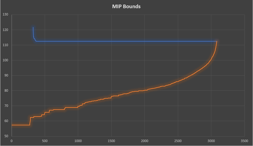 |
| Lower and upper bound. The upper bound is the best found solution. |
When we look at the blue line (best solution so far) we see that the solver had to do a bit of work to find a feasible integer solution. The first feasible solution was found after about 300 seconds. After that the objective quickly improved. After about 500 seconds not much was happening anymore: the solver just worked on tightening the lower bound (the best possible integer solution).
TSP relaxation
Note that if we drop the bounds related to the due and release dates and also ignore the precedence constraints, we end up with a pure TSP model. The TSP cost matrix looks like: \(c_{i,j} = \mathit{setup}_{i,j} + \mathit{proctime}_j\). The cost from the last job back to the initial job is set to zero. As expected this leads to a shorter makespan of 102.595:
 |
| Relaxed TSP solution |
The orange setup times are shorter than for the original model. Of course, as the processing times are constant, we might as well use for TSP costs: \(c_{i,j} = \mathit{setup}_{i,j}\). The optimal objective value will no longer be the total makespan but the optimal sequencing will be the same.
Solving this pure TSP model with TMZ formulation is very difficult and takes much more time than the 3000 seconds we needed for the scheduling model with the additional due date, release date and precedence constraints. These extra constraints make the problem easier (which is not that surprising). To be complete: I solved the TSP model using a very different formulation from [4] (this solved very quickly for this size).
Or-tools
A very fast way of solving this model is presented in [5]. Some notes:
- The fractional values have been scaled to make them integers. In most cases constraint solvers do not like floating point numbers. We may need to watch out for the integer range (some solver may support bigints).
- Preprocessing has been done to move parts of the setup time into the processing time. I.e. \[\begin{align} &\mathit{fixed}_j := \min_i \mathit{setup}_{i,j} \\ & \mathit{proctime}_j := \mathit{proctime}_j + {fixed}_j \\ & \mathit{setup}_{i,j} := \mathit{setup}_{i,j} - {fixed}_j\end{align}\]
References
- A. P. Burger, C. G. Jacobs, J. H. Vuuren, S. E. Visagie, Scheduling Multi-colour Print Jobs with Sequence-dependent Setup Times, J. of Scheduling, vol. 18, no. 2, 2015, pp. 131-14
- Orman, A. J. and Williams, H. Paul (2004) A survey of different integer programming formulations of the travelling salesman problem. Operational Research working papers, LSEOR 04.67
- Miller C.E., A.W. Tucker and R.A. Zemlin (1960) Integer programming formulation of travelling salesman problems, J. ACM, 3, 326–329.
- Unjust benchmark: TSP MIP/Gurobi vs GA/Octave, https://yetanothermathprogrammingconsultant.blogspot.com/2009/04/unjust-benchmark-tsp-mipgurobi-vs.html
- https://github.com/google/or-tools/blob/master/examples/python/single_machine_scheduling_with_setup_release_due_dates_sat.py
Hi Erwin, thank you for your formulation. I have a quastion about sequence dependency. Why did you use TSP formulation. Does not a formulation as below work? SETUP_ij + START_j + PROCESSTİME_j <= M*Xij or SETUP_ij + START_j + PROCESSTİME_j <= M*(1-Xij).
ReplyDeleteThat does not look correct at all.
DeleteSorry, I made a mistake. It is exactly as follows.
DeleteSETUP_ij + START_j + PROCESSTİME_j <= START_i + M*Xij or SETUP_ij + START_j + PROCESSTİME_j <= START_i + M*(1-Xij).
Sorry again, correct formulation is as follows. Let's say setup times are symetric.
DeleteSETUP_ij + START_j + PROCESSTİME_j <= START_i + M*Xij or SETUP_ij + START_i + PROCESSTİME_i <= START_j + M*(1-Xij).
Is'nt this formulation sufficient? Why did you use TSP formulation for setup times?
Dear Erwin, do you have any example for solving similar problem on multiple machine with job exclusions?
ReplyDeleteOur problem is just like the combination of this and another problem you have shared in another article. (https://yetanothermathprogrammingconsultant.blogspot.com/2019/06/machine-scheduling.html)
constraints:
Not all machines can do all jobs
Sequence Dependent Setup Times
object: minimize makespan or overall setup time
thank you so much.