Strange scheduling problem

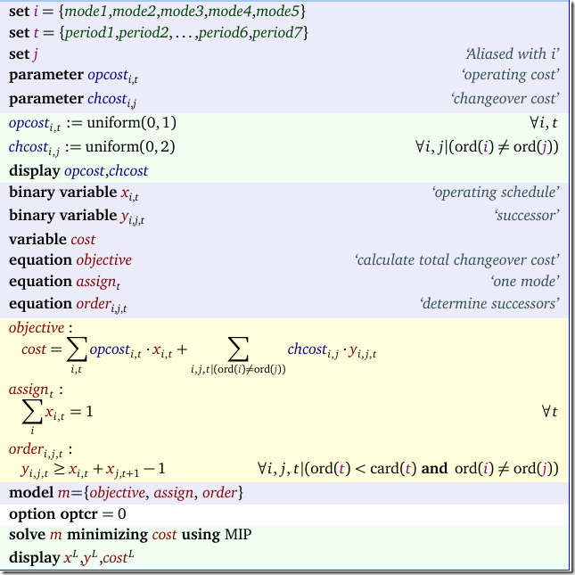
A somewhat strange scheduling model was presented to me. We operate a machine in one of several operating modes \(i\). We have time periods \(t\) and the operating cost \(c^{op}_{i,t}\) changes over time. Obviously, the best schedule would be to pick in each period \(t\) the cheapest operating mode. Now we add a changeover cost: when we change from mode \(i\) to mode \(j\) we pay some cost \(c^{ch}_{i,j}\). This would require a real optimization model to find the optimal operating sequence.

Here is a simple model to handle this:

We have used some random data here, which looks like:

----     12 PARAMETER opcost  operating cost           period1     period2     period3     period4     period5     period6     period7 mode1       0.172       0.843       0.550       0.301       0.292       0.224       0.350 mode2       0.856       0.067       0.500       0.998       0.579       0.991       0.762 mode3       0.131       0.640       0.160       0.250       0.669       0.435       0.360 mode4       0.351       0.131       0.150       0.589       0.831       0.231       0.666 mode5       0.776       0.304       0.110       0.502       0.160       0.872       0.265 ----     12 PARAMETER chcost  changeover cost             mode1       mode2       mode3       mode4       mode5 mode1                   0.572       1.188       1.445       1.256 mode2       0.928                   0.827       0.235       0.628 mode3       0.093       0.677                   0.364       1.291 mode4       1.121       1.540       0.596                   1.322 mode5       1.512       1.255       0.568       0.173

The solution looks like:

----     34 VARIABLE x.L  operating schedule           period1     period2     period3     period4     period5     period6     period7 mode1                                                           1           1           1 mode3           1           1           1           1 ----     34 VARIABLE y.L  successor                 period4 mode3.mode1           1 ----     34 VARIABLE cost.L                =        2.139

We see one changeover between periods 4 and 5. Notice that \(y\) is defined in the model above as:
\[y_{i,j,t} = \begin{cases} 1 \> \text{if $x_{i,t}=1$ and $x_{i,t+1}=1$} \\
                                      0 \> \text{otherwise}\end{cases}\]

This can also be interpreted as a nonlinear constraint \(y_{i,j,t} = x_{i,t}x_{i,t+1}\). In the model we have linearized this. A refinement of the model would have us look at the operating mode just before we start scheduling (i.e. the operating mode in period 0). To handle that easily it is helpful to change the definition of \(y\) to:
\[y_{i,j,t} = \begin{cases} 1 \> \text{if $x_{i,t-1}=1$ and $x_{i,t}=1$} \\
                                      0 \> \text{otherwise}\end{cases}\]

Only equation order needs to change:

Note that \(x0\) is an extremely sparse matrix: it has only one element corresponding to the operating mode for the machine just before period 1. (We used here a GAMS feature: addressing lags outside the domain cause the symbol to be dropped; so \(x_{i,t-1}\) for \(t=period1\) will disappear; in that special case the parameter \(x0\) will kick in). The final results with this initial changeover cost is:

----     37 VARIABLE x.L  operating schedule           period1     period2     period3     period4     period5     period6     period7 mode1                                                           1           1           1 mode3                                               1 mode4           1           1           1 ----     37 VARIABLE y.L  successor                 period4     period5 mode3.mode1                       1 mode4.mode3           1 ----     37 VARIABLE cost.L                =        2.438

Note that the initial mode in period 0 was 4, and now we keep operating using that mode for a little while.