The following is a well-know application of branch-and-bound: select the k best independent variables to include in the regression. Often best means: best residual sum of squares. When we use a slightly different objective we can let the solver decide on k instead of fixing k in advance.
The paper:
shows the detailed MIQP model:
We could easily reproduce some of their results in GAMS.
First we load the data into our familiar y and X arrays:
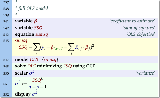
Then we first solve a full OLS to get an estimate of the variance. We need to use the level of the SSQ variable from the solution:
Finally we run the MIQP on the Cp criterion:
Note that the n is a constant, so we could drop it from the objective and find the same optimal solutions. We keep it to make the objective interpretable as the Mallow’s Cp quantity.
Many of the data sets used in the paper contain columns with categorical data. In regression models these are typically handled by a set of dummy variables. When using stepwise regression or a method like MIQP we probably should include (or exclude) a whole block of dummy variables (corresponding to the same categorical variable) instead of considering them individually for inclusion. That makes the MIQP model a bit more complicated to express (but easier to solve).
The housing data set used above had just a single dummy variable. In this case there is no problem. Indeed we can reproduce the results quite easily. From the paper:
We have:
using the formulas:
For problems with real categorical data (with more than two levels), we want to adjust the model. In this case we introduce nlevels-1 dummy variables. These dummies belong to the same “block” as they refer to the same categorical variable. We can adapt the MIQP model in two ways:
- Keep all j binary variables z and add equality constraints for the z’s belonging to the same block.
- Generate only z(k) binary variables and bound all the beta’s belonging to the same block by the same z(k). I.e. we need to map from beta(j) to z(k).
As the paper notices, when we use indicator constraints (Cplex, Xpress, SCIP), we could use implications so we don’t have to use a big-M constant
GAMS does not have language facilities to handle this (it allows indicator variables in a Cplex option file, but I feel uncomfortable if an option file – for tolerances and such things – changes the meaning of the model in such a substantial way). Ampl does this better by really having implications in the language.
I don’t really mind using big-M values. As these are essentially bounds on the decision variables, in practice we should be able to come up with a reasonable value.
Note
With some of the other data sets I am note sure how the paper arrives at their results. E.g. data set servo:
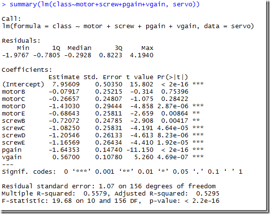
I.e. we have 4 independent variables, two of which are categorical (motor and screw, both with levels A through E). Pgain and vgain are numerical it looks like. The standard way to handle this in a regression model is to use 4 dummy variables each for the categorical variables motor and screw. Indeed this is what R does:
We see that level A does not generate a dummy variable (instead corresponds to all zeros in the other dummy variables B..E). Pgain and vgain are normal variables. I.e. we end up with a model with a total of p=10 variables (not counting the constant term).
In the paper however we see p=19:
My conjecture is that they did two things differently: the categorical variables are transformed using 5 dummy variables instead of 4; and the variables pgain and vgain are also considered as categorical variables and encoded using 4 and 5 dummies. It is interesting to see how even such a small data set can lead to confusion. How else can we arrive at p=19?


![image_thumb1[1] image_thumb1[1]](https://blogger.googleusercontent.com/img/b/R29vZ2xl/AVvXsEg3WVF-Eqv19z-MK7i-FTEdSP_wE_cGXXXChLsmjXUQbETI97nssPwKK6fUDYSFw-IdrPzkokYEhJ0ucGD1Zph6tcWkFoplsJg-R4Rg78FyX9TQ8MF3OjN9pVPeG3H2ChTxb8s0-PHKDJBz/?imgmax=800)


No comments:
Post a Comment