The Hostile Brothers Problem (1)

Another quadratic problem that has some interesting features – this is an old favorite of mine. The problem is stated as follows: a patriarch has n sons and wants to build them each a house on his estate such that the minimum distance between them is maximized. We assume here the parents plot is simply [0,1]x[0,1] and high fertility led to n=75 brothers.

When we random place the points we get a small minimum distance: 0.0088. The two orange points almost overlap.

When forming the objective function we can do two immediate tricks:

• We don’t need to compare all points i,j with each other twice. We can limit the distance calculations to the lower triangular part, i.e. were i > j.
• We can drop the sqrt in the distance calculation as this is a monotonic function.
• The default GAMS all-zero starting point is very bad: all gradients are zero. E.g. conopt will just stay at that point: it does not move an inch. Better is to use the above random configuration as initial point. From the results we see this is actually not a bad starting point.

There are two different objectives we can use. The first objective is a nice, compact single objective function that is unfortunately non-differentiable. The second formulation leads to a set of upper limits on mindist (we are maximizing mindist so we automatically find the correct one; note that mindist represents the squared minimum distance). The set lt(i,j) has 0.5(n²–n)=2775 elements, so we have 2775 inequalities in the second case.

Typically local NLP solvers like the second form better. E.g. with Conopt:

S O L V E      S U M M A R Y      MODEL   m1                  OBJECTIVE  mindist      TYPE    DNLP                DIRECTION  MAXIMIZE      SOLVER  CONOPT              FROM LINE  49 **** SOLVER STATUS     4 Terminated By Solver      **** MODEL STATUS      7 Feasible Solution         **** OBJECTIVE VALUE                0.0065

S O L V E      S U M M A R Y      MODEL   m2                  OBJECTIVE  mindist      TYPE    NLP                 DIRECTION  MAXIMIZE      SOLVER  CONOPT              FROM LINE  50 **** SOLVER STATUS     1 Normal Completion         **** MODEL STATUS      2 Locally Optimal           **** OBJECTIVE VALUE                0.0169

The second objective is much better although the model is much bigger, and we get a minimum distance of 0.1302. As you can see here, problem size is not all that matters when solving optimization problems. The brothers are now located as follows:

The orange points indicates where we observe the minimum distance. This starts to look like a grid we would expect. This also explains why we see an increase in the use of nonlinear programming in packing applications.

Next: towards global solutions.

Update: 3d version

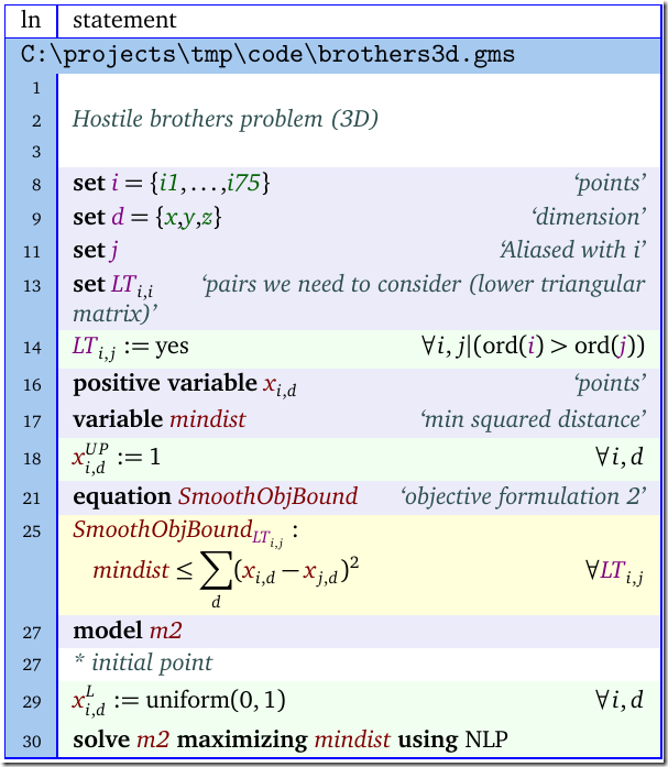
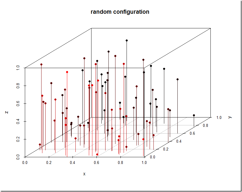
We can generalize to 3d as follows. The plots are somewhat difficult to understand.

Note: the red colors are related to the y-coordinate of the point.