Experiment: Database Diagram of GAMS model

It is always helpful to look at your model in a different way. Not sure if this is a very useful tool in practice. But it may help when passing on data from a GAMS model to a DBA as a documentation tool.

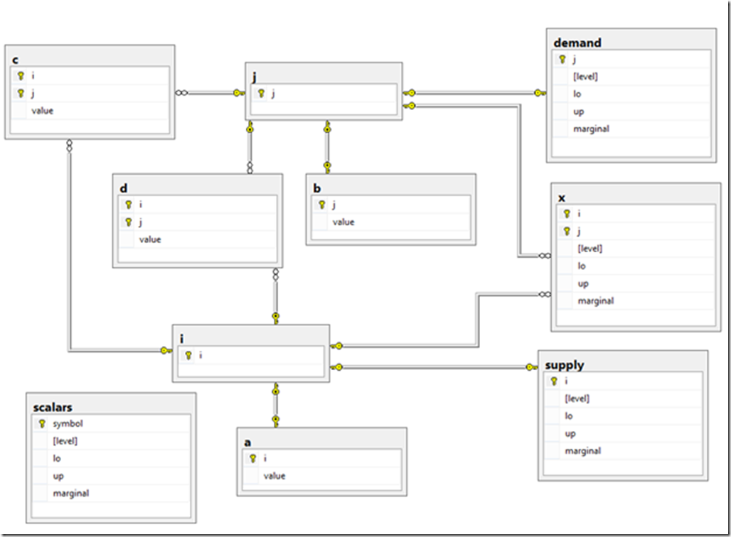
Sets        i   canning plants   / seattle, san-diego /        j   markets          / new-york, chicago, topeka / ;   Parameters        a(i)  capacity of plant i in cases          /    seattle     350               san-diego   600  /        b(j)  demand at market j in cases          /    new-york    325               chicago     300               topeka      275  / ;   Table d(i,j)  distance in thousands of miles                     new-york       chicago      topeka       seattle          2.5           1.7          1.8       san-diego        2.5           1.8          1.4  ;   Scalar f  freight in dollars per case per thousand miles  /90/ ;   Parameter c(i,j)  transport cost in thousands of dollars per case ;             c(i,j) = f * d(i,j) / 1000 ;   Variables        x(i,j)  shipment quantities in cases        z       total transportation costs in thousands of dollars ;   Positive Variable x ;   Equations        cost        define objective function        supply(i)   observe supply limit at plant i        demand(j)   satisfy demand at market j ;   cost ..        z  =e=  sum((i,j), c(i,j)*x(i,j)) ;   supply(i) ..   sum(j, x(i,j))  =l=  a(i) ;   demand(j) ..   sum(i, x(i,j))  =g=  b(j) ;   Model transport /all/ ;   Solve transport using lp minimizing z ;   Display x.l, x.m ;