Wednesday, October 12, 2016

Optimization: Retraction

image

We, the Editors and Publishers of Optimization: A Journal of Mathematical Programming and Operations Research, are retracting the following article:

Fridoun Moradlou and Sattar Alizadeh, Strong Convergence Theorem by a New Iterative Method for Equilibrium Problems and Symmetric Generalized Hybrid Mappings,http://www.tandfonline.com/doi/full/10.1080/02331934.2015.1032283

We are now aware of a substantially similar version of this article which was previously submitted to and published in Mediterranean Journal of Mathematics by the same authors:

Sattar Alizadeh and Fridoun Moradlou, A Strong Convergence Theorem for Equilibrium Problems and Generalized Hybrid Mappings, Mediterranean Journal of Mathematics, DOI: 10.1007/s00009-014-0462-6,http://link.springer.com/article/10.1007%2Fs00009-014-0462-6.

This action constitutes a breach of warranties made by the authors with respect to originality and of our policy on publishing ethics and integrity. We note we received, peer-reviewed, accepted, and published the article in good faith based on these warranties, and censure this action.

http://www.tandfonline.com/doi/full/10.1080/02331934.2015.1032283

Publishers seem to become more aggressive (may be assertive is a better word) about these things and retract more often. The web site http://retractionwatch.com/ offers some fascinating reading.

Update

See also the astonishing story here:

image

http://link.springer.com/article/10.1007/s10288-016-0329-8

Monday, October 10, 2016

One more P=NP proof?

image

Abtract. We present a polynomial-sized linear program (LP) for the \(n\)-city TSP drawing upon "complex flow" modeling ideas by the first two authors who used an \(O(n^9) \times O(n^8)\) model*. Here we have only \(O(n^5)\) variables and \(O(n^4)\) constraints. We do not model explicit cycles of the cities, and our modeling does not involve the city-to-city variables-based, traditional TSP polytope referred to in the literature as "The TSP Polytope." Optimal TSP objective value and tours are achieved by solving our proposed LP. In the case of a unique optimum, the integral solution representing the optimal tour is obtained using any LP solver (solution algorithm). In the case of alternate optima, an LP solver (e.g., an interior-point solver) may stop with a fractional (interior-point) solution, which (we prove) is a convex combination of alternate optimal TSP tours. In such cases, one of the optimal tours can be trivially retrieved from the solution using a simple iterative elimination procedure we propose. We have solved over a million problems with up to 27 cities using the barrier methods of CPLEX, consistently obtaining all integer solutions. Since LP is solvable in polynomial time and we have a model which is of polynomial size in \(n\), the paper is thus offering (although, incidentally) a proof of the equality of the computational complexity classes "P" and "NP". The non-applicability and numerical refutations of existing extended formulations results (such as Braun et al. (2015) or Fiorini et al. (2015) in particular) are briefly discussed in an appendix. [*: Advances in Combinatorial Optimization: Linear Programming Formulation of the Traveling Salesman and Other Hard Combinatorial Optimization Problems (World Scientific, January 2016).]

https://arxiv.org/abs/1610.00353

Unfortunately there are about as many \(P=NP\) proofs around as there are \(P\ne NP\) proofs. See (1) for a large list. The first author is already on the list with a few earlier papers.

As a practitioner, all of this may not be so important, but there are cases where I see complexity theory being somewhat misused or misunderstood in the following sense. When confronted with a combinatorial problem, a common reaction is to a-priori dismiss Mixed Integer Programming in favor of some heuristic, often accompanied with some mumblings about NP-hard problems. I believe complexity theory says very little about solving a given problem of a given size with an actual MIP solver. Notice also that many state-of-art MIP solvers contain many heuristics. In practice, for large difficult problems, MIP solvers can often (but not always) deliver good solutions quickly, with the added advantage of giving you an indication of how close we are from a possible optimal solution (the gap).

References

  1. Gerhard J. Woeginger, The P-versus-NP page, http://www.win.tue.nl/~gwoegi/P-versus-NP.htm

Saturday, October 8, 2016

An alternative linear programming solution technique

image

Abstract

Linear superiorization considers linear programming problems but instead of attempting to solve them with linear optimization methods it employs perturbation resilient feasibility-seeking algorithms and steers them toward reduced (not necessarily minimal) target function values. The two questions that we set out to explore experimentally are (i) Does linear superiorization provide a feasible point whose linear target function value is lower than that obtained by running the same feasibility-seeking algorithm without superiorization under identical conditions? and (ii) How does linear superiorization fare in comparison with the Simplex method for solving linear programming problems? Based on our computational experiments presented here, the answers to these two questions are: “yes” and “very well”, respectively.

http://www.optimization-online.org/DB_HTML/2016/10/5665.html


image

Abstract

Linear superiorization (abbreviated: LinSup) considers linear programming (LP) problems wherein the constraints as well as the objective function are linear. It allows to steer the iterates of a feasibilityseeking iterative process toward feasible points that have lower (not necessarily minimal) values of the objective function than points that would have been reached by the same feasiblity-seeking iterative process without superiorization. Using a feasibility-seeking iterative process that converges even if the linear feasible set is empty, LinSup generates an iterative sequence that converges to a point that minimizes a proximity function which measures the linear constraints violation. In addition, due to LinSup’s repeated objective function reduction steps such a point will most probably have a reduced objective function value. We present an exploratory experimental result that illustrates the behavior of LinSup on an infeasible LP problem.

http://www.optimization-online.org/DB_HTML/2016/10/5666.html

The Huffington Post and the Future of Statistical Computing

Via the Huffington Post copied from Quora:


How do you see statistical computing evolving over the next ten to twenty years?originally appeared on Quora: the knowledge sharing network where compelling questions are answered by people with unique insights.

Answer by Hadley Wickham, Chief Scientist, RStudio, on Quora:

“How do you see statistical computing evolving over the next ten to twenty years?”


“Prediction is very difficult, especially about the future.” - Niels Bohr. I probably shouldn’t answer this question because I’m likely to make predictions that will come back to haunt me. (In 2004, Bill Gates predicted that “spam will be a thing of the past in two years time.”) I’ll take a stab at it anyway:

  1. Open source and open science will continue to gain importance. It will become increasingly difficult for closed source statistical environments to survive.
  2. We are likely to see at least one alternative implementation to R that has substantially better performance. The most promising candidate at this time is rho.
  3. Data storage tools (like databases) will continue to gain more stat/ML tools. The needs of data science will drive much innovation in database space over the next ten years.
  4. A new generation of tools (including both IDEs and ML algorithms) will more fluently combine the strengths of humans and computers.

Thursday, October 6, 2016

Scheduling Business Dinners: an MINLP, MIQCP and MIP model

In (1) a problem is discussed where an optimization model can help us.

We want to set up \(N\) business dinners attended by customers and suppliers with the following peculiarities:

  • there are \(T\) tables,
  • we need to seat \(C\) customers and \(S\) suppliers,
  • at most \(Maxc\) customers and at most \(Maxs\) suppliers can sit at a single table,
  • a customer \(c\) and supplier \(s\) must sit at the same table exactly once,
  • two suppliers can only sit at the same table at most once

We want to minimize the number of dinners \(N\) we need to organize such that all these constraints are met.


Restaurant Flo in Barcelona, Spain [link]

The data

We use the example data from (1):

  • 6 customers, 5 suppliers
  • \(Maxc=3\), \(Maxs=2\)
  • 2 tables

A (non-optimal) solution with 8 dinner rounds is given:

image

An MINLP model

We start with our central binary variable \(x_{i,t,n}\in\{0,1\}\) indicating if person \(i\) sits at table \(t\) in dinner round \(n\). With this we can develop a Mixed Integer Nonlinear Programming model:

\[\boxed{\begin{align}
\min\>&\sum_n y_n && && \text{minimize number of dinner rounds} \\
        &\sum_t x_{i,t,n} \le 1 &&\forall i,n&&\text{sit at one table}\\
        &\sum_s x_{s,t,n} \le Maxs &&\forall t,n&&\text{limit suppliers at table}\\
        &\sum_c x_{c,t,n} \le Maxc &&\forall t,n&&\text{limit customers at table}\\
      * \> &\sum_{t,n} x_{c,t,n}\cdot x_{s,t,n} = 1&&\forall c,s&&\text{customers and suppliers meet exactly once}\\
     * \> &\sum_{t,n} x_{s1,t,n} \cdot x_{s2,t,n} \le 1&&\forall s1\ne s2&&\text{suppliers sit at most once at the same table}\\
     * \> &y_n = \max_{i,t} \{x_{i,t,n}\} && \forall n &&\text{we need a dinner round}\\
       &x_{i,t,n},y_n \in \{0,1\}
\end{align}}\]

The equations marked with a * are nonlinear. The variable \(y_n\) indicates whether we need a dinner round \(n\).


A non-convex MIQCP model

To implement the above MINLP we can apply a few modifications:

  • When we checked if suppliers \(s1,s2\) are at the same table, we can skip checking \(s2,s1\). Hence we only need to check suppliers \(s1,s2\) with \(s1<s2\). This saves us a number of equations.
  • The constraint \(y_n = \max_{i,t} \{x_{i,t,n}\}\) can be written as a collection of inequalities \(y_n \ge x_{i,t,n}\) (we use the objective to help us drive down \(y_n\)).
  • Optionally we can require that \(y_n \ge y_{n+1}\), This makes the solutions more readable (we have the used dinner rounds first) but also reduces symmetry.
  • There are more symmetries in the model we can try to alleviate. E.g. order dinner rounds and order tables by some statistic.

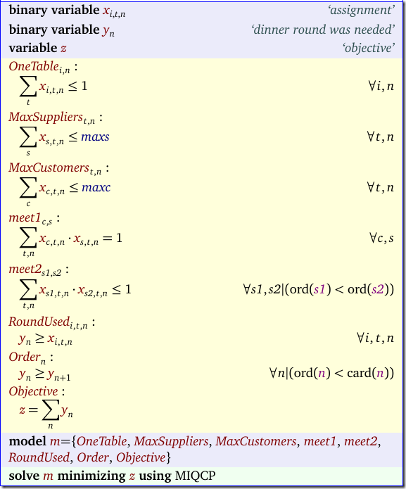
We are now only left with quadratic terms in the constraints. Such a model is called a Mixed Integer Quadratically Constrained Problem (MIQCP). Although solvers like Cplex and Gurobi can solve convex MIQCPs, unfortunately this problem is non-convex. That means we need a global solver. The model below can be solved quickly with the solvers GloMIQO, Antigone and Baron. Interestingly, the global solver Couenne is struggling mightily with this model: it has troubles finding a feasible solution.
image

A linearized MIP model

The binary multiplication can be linearized using a standard reformulation:

\[\begin{matrix}
\boxed{\begin{align}&z=x\cdot y\\
                             &x,y,z\in \{0,1\}\end{align}}&\Longleftrightarrow&
\boxed{\begin{align}&z \le x\\&z \le y\\&z\ge x+y-1\\&x,y,z\in \{0,1\}\end{align}}
\end{matrix}\]

Note that we need to apply this reformulation on the individual product terms in the two quadratic constraints. This means we need to introduce a number of additional variables in the model.

We can simplify the binary multiplication further in the supplier case: we only need to make sure that \(z \ge x+y-1\). That will save us some constraints. The reason hat we can do this is that we have an inequality of the form \(\sum_i x_i \cdot y_i \le 1\) so we are only interested in the product terms that are forced to be one. Hence we have the two different cases:

\[\begin{matrix} \displaystyle\sum_i x_i\cdot y_i = 1 & \Longrightarrow &
\boxed{\begin{align} &z_i \le x_i\\ &z_i \le y_i\\&z_i \ge x_i+y_i-1\\&\sum_i z_i=1\end{align}}\\
\displaystyle\sum_i x_i\cdot y_i \le 1 & \Longrightarrow &
\boxed{\begin{align}&z_i \ge x_i+y_i-1\\&\sum_i z_i\le 1 \end{align}}\end{matrix}\]

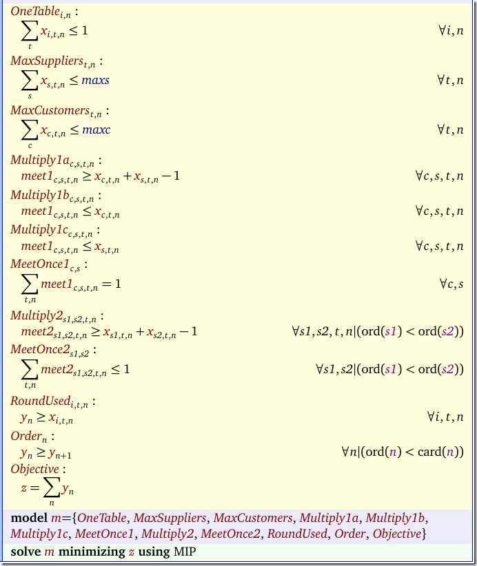
I should note that I assume \(x_i,y_i,z_i \in \{0,1\}\). It is nice to see both constructs next to each other in one small model. The complete linearized model can look like:  

image

image

This model can now be solved with any MIP solver, including Cplex and Gurobi which were out of the picture for the MIQCP model formulation.

An optimal solution with 3 dinner rounds is:

image


References

  1. Alejandra Estanislao, Frédéric Meunier, “A Business Dinner Problem”, Journal of Combinatorial Mathematics and Combinatorial Computing, 97, 173-188, 2016. [link]

Tuesday, October 4, 2016

Optimal Opera Seating: a MIP formulation

Here is an interesting problem that is somehow not so easy to model as a Mixed Integer Programming (MIP) problem:

So i have an opera houses with 10 rows and 10 columns of seats (Total :100). Each seat is allocated a preference value Aij. The preference value is halved if the group do not get seats in same row. Eg: If a reservation in opera house is for 5 people and only 2 can be accommodated in top row and 3 in next row, the preference value is actually halved for each seat. There are total of n reservations with 'n' > 100 seats. What will the best way to maximize the customer preference (n *Aij).If it can be done by linear programming, how should the equation look like.


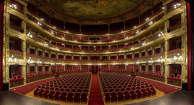
Interior of Teatro de Romea in Murcia, Spain (link)

The data

I assume we have a set of groups \(g\) and their sizes: \(size_g\). A couple would be a group of size 2. Further use the rule that only complete groups can be seated (i.e. no partial groups).

The seats are organized as a grid \((i,j)\) where \(i\) is the row and \(j\) is the column. Each seat has a “preference value” \(a_{i,j}\).

A simpler case: assignment

Let’s first ignore the difficulty about single or multiple row assignments. Without this complication we are essentially dealing with an assignment problem:

\[\boxed{\begin{align}
\max\>&\sum_{i,j,g} a_{i,j} x_{i,j,g}\\
&\sum_g x_{i,j,g} \le 1 \>\>\forall i,j\\
&\sum_{i,j} x_{i,j,g} = \mathit{place}_g \cdot \mathit{size}_g \>\>\forall g\\
&x_{i,j,g} \in \{0,1\}\\
&\mathit{place}_g \in \{0,1\}
\end{align}}\]

Here \(x_{i,j,g}=1\) if a member of group \(g\) is seated in location \((i,j)\). The binary variable \(\mathit{place}_g\) indicates whether we accommodate group \(g\) (and thus seat all its members).

This model works both for the case where \(n=\sum_g \mathit{size}_g\) exceeds the number of available seats or when \(n\) is a smaller number.

This is quite easy. However using random \(a_{i,j}\) we see groups scattered around the rows:

image

The numbers in each cell are the group IDs.

The tough case: penalize multiple row assignments

I am not sure if this is the best or even a good formulation. What I did is introduce a new index \(r = \{\text{OneRow},\text{MultipleRows}\}\). Then my main variables are \(x_{i,j,g,r} \in \{0,1\}\). Here is the complete model:

image

The parameter pref2 was populated as:

image

Admittedly: this model is not very straightforward and obvious. I am curious if there are better formulations.

The results look ok: there is a heavy preference for placing groups in the same row:

image

I would guess a constraint Programming (CP) approach may make it easier to model this problem.

Sunday, October 2, 2016

Matlab vs GAMS: Integer Programming

In a previous post I translated a small GAMS model (model number one from the GAMS model library) into Matlab and compared the codes side-by-side. In this post we take slightly more complicated MIP model written in Matlab and convert it into GAMS.   

The problem discussed here (1) involves a network of factories, warehouses and sales outlets. We need to find the least expensive flow of products from factories to warehouses to stores. One particularity is that each store gets its products from one warehouse.

Mathematical Model

We use the following indices:

  • \(p\): products
  • \(f\): factories
  • \(w\): warehouses
  • \(s\): stores

We introduce the following variables:

  • \(x_{p,f,w} \ge 0\): shipments of product \(p\) from factory \(f\) to warehouse \(w\),
  • \(y_{s,w} \in \{0,1\}\): links each store \(s\) to a single warehouse \(w\).

The data associated with the model is:

  • \(pcost_{f,p}\): unit production cost
  • \(tcost_{p}\): unit transportation cost
  • \(dist_{f,w}, dist_{s,w}\): distances
  • \(pcap_{f,p}\): factory production capacities
  • \(wcap_{w}\): warehouse capacity
  • \(d_{s,p}\): demand for product \(p\) at store \(s\)
  • \(turn_{p}\): product turnover rate

The optimization model looks like:

\[\boxed{\begin{align}
\min&\sum_{p,f,w} (pcost_{f,p}+tcost_p\cdot dist_{f,w})\cdot x_{p,f,w}+\sum_{s,w,p} d_{s,p}\cdot tcost_p \cdot dist_{s,w} \cdot  y_{s,w}\\
&\sum_w x_{p,f,w} \le pcap_{f,p} \>\>\forall f,p \>\> \text{(production capacity)}\\
&\sum_f x_{p,f,w} = \sum_s d_{s,p}\cdot  y_{s,w} \>\>\forall p,w \>\>\text{(demand)}\\
&\sum_{p,s} \frac{d_{s,p}}{turn_{p}} y_{s,w} \le wcap_{w}\>\>\forall w \>\>\text{(warehouse capacity)}\\
&\sum_w y_{s,w} = 1\>\>\forall s \>\>\text{(one warehouse for a store)}\\
&x_{p,f,w} \ge 0 \\
&y_{s,w} \in \{0,1\}
\end{align}}\]

Matlab vs GAMS Implementation

Here we compare the Matlab implementation from (1) to a GAMS transcription of the model.

Matlab code GAMS code

rng(1) % for reproducibility

N = 20; % N from 10 to 30 seems to work. Choose large values with caution.

N2 = N*N;

f = 0.05; % density of factories

w = 0.05; % density of warehouses

s = 0.1; % density of sales outlets


F = floor(f*N2); % number of factories

W = floor(w*N2); % number of warehouses

S = floor(s*N2); % number of sales outlets


sets
  k
'locations' /factory1*factory20,
           warehouse1*warehouse20,store1*store40/

  f(k)
'factories' /factory1*factory20/
  w(k)
'warehouses' /warehouse1*warehouse20/
  s(k)
'stores' /store1*store40/

;

xyloc = randperm(N2,F+W+S); % unique locations of facilities

[xloc,yloc] = ind2sub([N N],xyloc);
Pick unique locations on a grid
Not 100% the same: just random locations. No guarantee of uniqueness.

parameters xloc(k),yloc(k);
xloc(k) = uniformint(1,20);
yloc(k) = uniformint(1,20);

P = 20; % 20 products


% Production costs between 20 and 100

pcost = 80*rand(F,P) + 20;


% Production capacity between 500 and 1500 for each product/factory

pcap = 1000*rand(F,P) + 500;


% Warehouse capacity between P*400 and P*800 for each product/warehouse

wcap = P*400*rand(W,1) + P*400;


% Product turnover rate between 1 and 3 for each product

turn = 2*rand(1,P) + 1;


% Product transport cost per distance between 5 and 10 for each product

tcost = 5*rand(1,P) + 5;


% Product demand by sales outlet between 200 and 500 for each

% product/outlet

d = 300*rand(S,P) + 200;


set p 'products' /product1*product20/;
parameters

   pcost(f,p)
'unit production cost'
   pcap(f,p)
'production capacity'
   wcap(w)
'warehouse capacity'
   turn(p)
'product turnover rate'
   tcost(p)
'unit transportation cost'
   d(s,p)
'demand'
;
pcost(f,p) = uniform(20,100);
pcap(f,p) = uniform(500,1500);
wcap(w) = uniform(400*
card(p),800*card
(p));
turn(p) = uniform(1,3);
tcost(p) = uniform(5,10);
d(s,p) = uniform(200,500);


distfw = zeros(F,W); % Allocate matrix for factory-warehouse distances

for ii = 1:F

    for jj = 1:W

        distfw(ii,jj) = abs(xloc(ii) - xloc(F + jj)) +

            abs(yloc(ii) - yloc(F + jj));

    end

end


distsw = zeros(S,W); % Allocate matrix for sales outlet-warehouse distances

for ii = 1:S

    for jj = 1:W

        distsw(ii,jj) = abs(xloc(F + W + ii) - xloc(F + jj))

            + abs(yloc(F + W + ii) - yloc(F + jj));

    end

end

 
The indexing is cleaner thanks to \(f,s,w\) being subsets of \(k\).

parameters
   distfw(f,w)
'distance factory-warehouse'
   distsw(s,w)
'distance store-warehouse'

;
distfw(f,w) = abs(xloc(f)-xloc(w))+abs(yloc(f)-yloc(w));
distsw(s,w) = abs(xloc(s)-xloc(w))+abs(yloc(s)-yloc(w));

obj1 = zeros(P,F,W); % Allocate arrays

obj2 = zeros(S,W);

% Generate the entries of obj1 and obj2.

for ii = 1:P

    for jj = 1:F

        for kk = 1:W

            obj1(ii,jj,kk) = pcost(jj,ii) + tcost(ii)*distfw(jj,kk);

        end

    end

end


for ii = 1:S

    for jj = 1:W

        obj2(ii,jj) = distsw(ii,jj)*sum(d(ii,:).*tcost);

    end

end

% Combine the entries into one vector.

obj = [obj1(:);obj2(:)]; % obj is the objective function vector

 
  positive variable x(p,f,w) 'flow factory to warehouse';
binary variable y(s,w) 'assign warehouse to store'
;
variable z 'objective variable'
;

equation obj 'objective'
;
obj..
  z =e=
sum
((p,f,w), (pcost(f,p)+tcost(p)*distfw(f,w))*x(p,f,w))
        +
sum
((s,w,p), d(s,p)*tcost(p)*distsw(s,w)*y(s,w));

matwid = length(obj);


Aineq = spalloc(P*F + W,matwid,P*F*W + S*W); % Allocate sparse Aeq

bineq = zeros(P*F + W,1); % Allocate bineq as full


% Zero matrices of convenient sizes:

clearer1 = zeros(size(obj1));

clearer12 = clearer1(:);

clearer2 = zeros(size(obj2));

clearer22 = clearer2(:);


% First the production capacity constraints

counter = 1;

for ii = 1:F

    for jj = 1:P

        xtemp = clearer1;

        xtemp(jj,ii,:) = 1; % Sum over warehouses for each product and factory

        xtemp = sparse([xtemp(:);clearer22]); % Convert to sparse

        Aineq(counter,:) = xtemp'; % Fill in the row

        bineq(counter) = pcap(ii,jj);

        counter = counter + 1;

    end

end

Matrix Aineq holding the coefficients for the inequality constraints is large and sparse, so use a sparse matrix instead of a dense one.   
 

equation prodcap(f,p) 'production capacity';
prodcap(f,p)..
   
sum
(w,x(p,f,w)) =l= pcap(f,p);

% Now the warehouse capacity constraints

vj = zeros(S,1); % The multipliers

for jj = 1:S

    vj(jj) = sum(d(jj,:)./turn); % A sum of P elements

end


for ii = 1:W

    xtemp = clearer2;

    xtemp(:,ii) = vj;

    xtemp = sparse([clearer12;xtemp(:)]); % Convert to sparse

    Aineq(counter,:) = xtemp'; % Fill in the row

    bineq(counter) = wcap(ii);

    counter = counter + 1;

end


equation whcap(w) 'warehouse capacity';
whcap(w)..
 
sum
((p,s),(d(s,p)/turn(p))*y(s,w)) =l= wcap(w);

Aeq = spalloc(P*W + S,matwid,P*W*(F+S) + S*W); % Allocate as sparse

beq = zeros(P*W + S,1); % Allocate vectors as full


counter = 1;

% Demand is satisfied:

for ii = 1:P

    for jj = 1:W

        xtemp = clearer1;

        xtemp(ii,:,jj) = 1;

        xtemp2 = clearer2;

        xtemp2(:,jj) = -d(:,ii);

        xtemp = sparse([xtemp(:);xtemp2(:)]'); % Change to sparse row

        Aeq(counter,:) = xtemp; % Fill in row

        counter = counter + 1;

    end

end

Matrix Aeq is for the coefficients of the equality constraints. Also stored as a sparse matrix
 

equation demand(p,w);
demand(p,w)..
  
sum(f,x(p,f,w)) =e= sum
(s, d(s,p)*y(s,w));

% Only one warehouse for each sales outlet:

for ii = 1:S

    xtemp = clearer2;

    xtemp(ii,:) = 1;

    xtemp = sparse([clearer12;xtemp(:)]'); % Change to sparse row

    Aeq(counter,:) = xtemp; % Fill in row

    beq(counter) = 1;

    counter = counter + 1;

end


equation assign(s) 'assign wh to store';
assign(s)..
  
sum
(w,y(s,w)) =e= 1;

intcon = P*F*W+1:length(obj);

lb = zeros(length(obj),1);

ub = Inf(length(obj),1);

ub(P*F*W+1:end) = 1;

[solution,fval,exitflag,output] = intlinprog(obj,intcon,Aineq,bineq,Aeq,beq,lb,ub);


model m /all/;
option
optcr=0;
solve
m minimizing z using mip;

The conclusion is that when we compare an equation based modeling system compared to a matrix based system, the equation based formulation is really more compact and readable when the model equations become more complex.

References