Monday, November 21, 2016

Cord Diagrams in R

image

A nice Cord Diagram produced with just two statements in R (see (1)):

par(mar = c(1, 1, 1, 1), bg="violetred4")
circlize::chordDiagram(matrix(1, 20, 20),
                       col="white",
                       symmetric = TRUE,
                       transparency = 0.85,
                       annotationTrack = NULL)

A collection of more meaningful graphs is in (2). Particularly impressive is:


References
  1. https://fronkonstin.com/2016/08/22/the-breathtaking-1-matrix/
  2. http://zuguang.de/circlize/

Friday, November 18, 2016

Constrained Least Squares solution times II

In this post I discussed a somewhat large linearly constrained least squares problem:

\[\begin{align}\min_P\>\>&||P s - f||^2\\ & \sum_i p_{i,j}\le 1\\ & p_{i,j} \ge 0 \end{align}\]

Note that \(i\) has 39 elements and \(j\) has 196 elements. We can solve this as a Quadratic Programming (QP) problem:

\[\begin{align}\min_x\>\>&x^TQx +c^Tx\\&Ax \{\le,=,\ge\} b\\&\ell\le x \le u\end{align}\]

There are two obvious ways to implement this. It is not immediately clear to me which one is best.

Formulation I
\[\boxed{\begin{align}\min_{P}\>&\sum_i \left(\sum_j p_{i,j} s_j – f_i \right)^2\\ & \sum_i p_{i,j} \le 1 \\ &p_{i,j} \ge 0 \end{align}}\]

For our data set this leads to a QP problem with 7644 variables and 196 linear constraints. The number of nonzero element in the lower triangle of the (quadratic) Q matrix is 401544. 

Formulation II 

\[\boxed{\begin{align}\min_{P,e}\>&\sum_i e_i^2\\ & \sum_j p_{i,j} s_j = f_i + e_i\\ &\sum_i p_{i,j} \le 1 \\ &p_{i,j} \ge 0 \end{align}}\]

Here we made the model substantially larger: we added variables \(e_i\) (the residuals) and we added (linear) constraints. Note that we created a pretty dense block here. However the Q matrix becomes much simpler: it is now a diagonal matrix. The statistics are: 7683 variables, 235 linear constraints and only 39 diagonal elements in Q.

We moved complexity from the nonlinear objective into the linear constraints. That sounds like a good thing. But we increased the number of variables, equations and nonzero-elements. The trade-off is not obvious.

Some results
Model Solver Time (sec) Notes
I Cplex 0.16 Warning:  diagonal perturbation of 1.5e-008 required to create PSD Q.
Warning:  Barrier optimality criterion affected by large objective shift.
II Cplex 0.08  
I IPOPT with MUMPS linear solver >1000 Could not solve in 1000 seconds. Messages:
MUMPS returned INFO(1) = -9 and requires more memory, reallocating.  Attempt 1
  Increasing icntl[13] from 1000 to 2000.
MUMPS returned INFO(1) = -9 and requires more memory, reallocating.  Attempt 2
  Increasing icntl[13] from 2000 to 4000.

Looks like IPOPT has some severe problems recovering after a reallocation (may be a bug).
II IPOPT with MUMPS linear solver 0.6  
I IPOPT with MA27 linear solver 200  
II IPOPT with MA27 linear solver 0.2  

The timings are seconds spend inside the solver doing real work (excluding model generation and solver reading and setup times). Indeed it looks like formulation II gives better performance and reliability. It is noted that the set \(i\) is small compared to \(j\) which makes this dataset somewhat unusual.

References
  1. http://yetanothermathprogrammingconsultant.blogspot.com/2016/11/constrained-least-squares-solution-times.html

Thursday, November 17, 2016

Constrained Least Squares solution times

In this post a somewhat larger linearly constrained least squares problem is solved using R. The problem is simply:

\[\begin{align}\min_P&||P s - f||^2\\ & \sum_i p_{i,j}\le 1\\ & p_{i,j} \ge 0 \end{align}\]

To make things easier for the QP solver I implemented the model (in GAMS) as:

\[\begin{align}\min_{P,e}&\sum_i e_i^2\\ & \sum_j p_{i,j} s_j = f_i + e_i\\ &\sum_i p_{i,j} \le 1 \\ &p_{i,j} \ge 0 \end{align}\]

The timings for a problem with \(39 \times 196\) elements in \(P\) are:

R+constrOptim 15 hours
R+auglag 2 hours
GAMS+IPOPT 1.2 seconds
GAMS+Cplex 0.15 seconds

Cplex uses a specialized convex quadratic solver, while IPOPT is a general purpose NLP (nonlinear programming) solver.

Sometimes it helps to choose the right solver for the problem at hand.

References
  1. Follow-up on this blog detailing the effects on my reformulation is here: http://yetanothermathprogrammingconsultant.blogspot.com/2016/11/constrained-least-squares-solution.html

Monday, November 14, 2016

Taxicab distances: L1 norm minimization

From this post:

Suppose we are given \(n\) points \(A_1, \dots, A_n \in \mathbb{R}^2\). The task is to find a point \(x = (x_1,x_2) \in \mathbb{R}^2\) such that the sum of distances to the points \(A_1, \dots, A_n\) in the \(\ell_1\)-norm is minimized. Formulate this problem as a linear program.

There are at least two (primal) formulations. A variable splitting technique can look like:

\[\boxed{\begin{align}
  \min & \sum_{i,j} y^+_{i,j} + y^-_{i,j}\\
  &y^+_{i,j} - y^-_{i,j} = x_j-A_{i,j}\\
  &y^+_{i,j}\ge 0, y^-_{i,j}\ge 0
\end{align}}\]

A different formulation is

\[\boxed{\begin{align}
  \min & \sum_{i,j} y_{i,j}\\
  &-y_{i,j} \le x_j-A_{i,j} \le y_{i,j}\\
  &y_{i,j}\ge 0
\end{align}}\]

I don’t think this formulation has a name. We can drop \(y_{i,j}\ge 0\) if we want, as this is implied by \(-y_{i,j}\le y_{i,j}\).

If you let mathematicians loose on this, you may end up with formulation 2 stated as:

\[\boxed{\begin{array}{ll} \text{minimize} & 1_{2n}^{\top} \mathrm y\\ \text{subject to} & -\mathrm y \leq (1_n \otimes \mathrm I_2) \, \mathrm x - \mbox{vec} (\mathrm A) \leq \mathrm y\\ & \mathrm y \geq 0_{2n}\end{array}}\]

I don’t really like this type of notation: at least for me it is much less intuitive.

The first formulation has fewer equations but more variables. The second formulation has more constraints as we need to split \(-y_{i,j} \le x_j-A_{i,j} \le y_{i,j}\) into \(x_j-A_{i,j} \ge –y_{i,j}\) and \(x_j-A_{i,j} \le y_{i,j}\). I don’t think there is much reason to choose one formulation above the other. Depending largely on my mood I use either version 1 or 2.

Thursday, November 10, 2016

Programming in R books

The following books emphasize the language features of R (opposed to applications such as statistics, machine learning or visualization).

Introduction

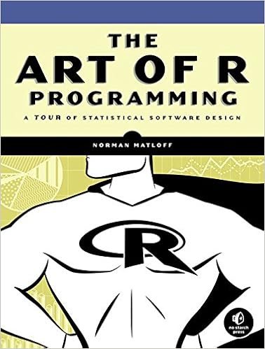
Norman Matloff, The Art of R Programming: A Tour of Statistical Software Design, No Starch Press; 1 edition (October 15, 2011)

[Amazon

Advanced

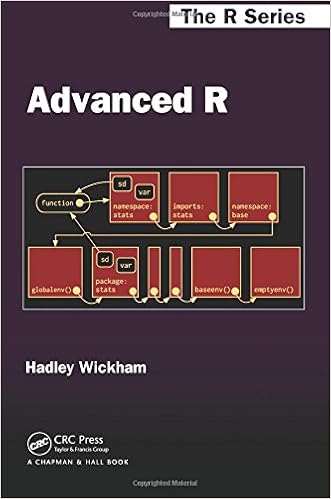
Hadley Wickham, Advanced R, Chapman and Hall/CRC; 1 edition (September 25, 2014)

[Amazon]
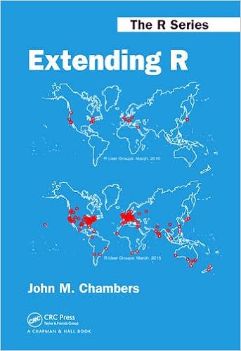
John M. Chambers, Extending R, Chapman and Hall/CRC (May 24, 2016)

[Amazon]


Special Topics

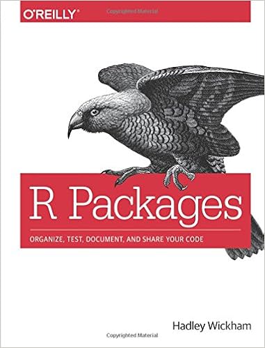
Hadley Wickham, R Packages: Organize, Test, Document, and Share Your Code, O'Reilly Media; 1 edition (April 13, 2015)

[Amazon]

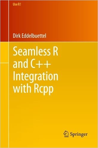
Dirk Eddelbuettel, Seamless R and C++ Integration with Rcpp, Springer; 2013 edition (June 4, 2013)

[Amazon]

Wednesday, November 9, 2016

NAG Optimization Modelling Suite

It looks to be like a somewhat low level unified subroutine interface to their optimization routines. The name “Optimization Modelling Suite” suggests to me something higher level, targeting more modeling opposed to programming. (I believe modeling and programming are overlapping but different paradigms).

From http://blog.nag.com/2016/11/the-new-nag-optimization-modelling-suite.html:

The New NAG Optimization Modelling Suite

Nowadays a vast majority of optimization solvers can handle very complex problems involving many variables and various types of the constraints with a different structure. Designing an interface for such a solver, which would allow a complex input without compromising the ease of use, is challenging.
A new suite of routines, the NAG Optimization Modelling Suite, has been introduced in Mark 26 of the NAG Library to tackle the input of complex problems without forming difficult interfaces with a daunting number of arguments. The suite is used by the new optimization solvers introduced at this mark; the semidefinite programming solver and the interior point method for nonlinear optimization. The suite will expand in the years to come to handle more problem types.
The main aim of the NAG Optimization Modelling Suite is the ability to define and solve various optimization problems in a uniform manner.
There are three key features of the suite. Firstly, the definition of the optimization problem and the call to the solver have been separated in such a way that the formulation of the problem is solver agnostic, i.e., the same problem can be set up in the same way for different solvers. Secondly, the problem representation is built up from basic components (for example, a QP problem is composed of a quadratic objective, simple bounds and linear constraints), therefore different types of problems reuse the same routines for their common parts. Finally, the call to the solver is notably simplified thanks to the fact that most of the information has already been provided.
The suite can be found in Chapter E04 of the NAG Library, mainly as e04r and e04s routines. There are many examples accompanying the routines of the suite to demonstrate the best practice.

Last time I used NAG was on a machine called CDC Cyber 170-750, something like:

Tuesday, November 8, 2016

Pyomo: Fancy Movie


R&D 100, 2016: Pyomo 4.0 - Python Optimization Modeling Objects [link]

Sunday, November 6, 2016

Excel Recalculation: Fixed Point Iterations

When we have circular references in our Excel spreadsheet, we can have Excel do a (large) number of iterations in the hope this converges to a solution. Mathematically speaking we could say this is like:

\[x_{i,j} := f_{i,j}(X)\]

where \(x_{i,j}\) is the cell in row \(i\) and column \(j\). This will converge to a fixed point:

\[X = F(X)\]

if the stars are aligned. Of course we can look at this as if we are solving a system of non-linear equations:

\[G(X)=F(X)-X=0\]

For a project, I am looking at some spreadsheets that have a few hundred thousand of such formulas.

Convergence can be a problem for a scheme like this. Below is a nice example of solving the equation \(x^2-x-1=0\) using two different fixed point iteration schemes:

  1. \(x_{(k+1)} := 1 +\displaystyle\frac{1}{x_{(k)}}\), this one converges
  2. \(x_{(k+1)} := \displaystyle\frac{1}{x_{(k)}-1}\), this one diverges
  3. \(x_{(k+1)} :=  x^2_{(k)} - 1\), also diverges

Details in the YouTube video below:

Note that we can interpret a Newton algorithm as a fixed point iteration:

\[x_{(k+1)} := x_{(k)} – \frac{f(x_{(k)})}{f’(x_{(k)})}\]

See (2) and (3) for more information how Excel does these recalculations.

References

  1. Oscar Veliz, Fixed point Iteration, https://www.youtube.com/watch?v=OLqdJMjzib8
  2. Recalculation in Excel 2002, https://msdn.microsoft.com/en-us/library/aa140058
  3. Multithreaded recalculation in Excel, https://msdn.microsoft.com/en-us/library/office/bb687899.aspx

Thursday, November 3, 2016

Microsoft Power BI and R

I noticed in the menu:

image

There is some info online:

It is interesting to see how Microsoft is embracing R.