Thursday, January 29, 2015

MS Visual-R

Microsoft has purchased Revolution (an R company). Here are some reactions:

Some thoughts:

  1. MS has already R inside Azure-ML. https://studio.azureml.net/
  2. I always thought of ML (Machine Learning) as a somewhat smallish but highly fashionable subset of Statistics, but now it seems ML is hyped so much to completely obscure Statistics.
  3. Is ML really that big?
  4. ML has little bit more of a CS and IT background (traditional statistics more of a math background with perhaps most applications in the social sciences?). May be CS/IT people are much better in their public relations. Also many companies nowadays see IT as core business, so may be there is more funding available for doing significant ML applications.
  5. MS has a poor performance record wrt analytics: poor Solver Foundation was abandoned in a bad way leaving some clients hanging to dry.
  6. MS already has a popular statistics package (it is called Excel). (Joking!)
  7. MS is a little bit late: IBM purchased SPSS in 2009.
  8. R is very successfully riding this hype cycle. Not bad for a somewhat funky and older language (rooted in S).
  9. Do we get an R.NET?
  10. TIBCO offers a commercial re-implementation of R.
  11. ML vs Statistics: http://brenocon.com/blog/2008/12/statistics-vs-machine-learning-fight/

Monday, January 26, 2015

The Hostile Brothers Problem (3)

Follow up on http://yetanothermathprogrammingconsultant.blogspot.com/2015/01/the-hostile-brothers-problem-1.html and http://yetanothermathprogrammingconsultant.blogspot.com/2015/01/the-hostile-brothers-problem-2.html.

Now some experiments that did not work.

Find global solutions with Baron

This is a very difficult job. One idea that may help is to add some symmetry breaking constraints:

image

This can reduce the search space considerably. We run the equation over all i–1: in GAMS this is notation that means we drop the first possible equation (the equation related to ord(i)=1).

In addition we can pass on a good solution we found with techniques described earlier. Unfortunately this helps but not enough to bring us close to proving global optimality:

  Iteration    Open nodes       Total time    Lower bound      Upper bound
          1             1        000:00:01     0.100000E-08     2.00000   
          1             1        000:00:07     0.200000E-08     2.00000   
*         2             2        000:00:10     0.163965E-01     2.00000   
*         2             2        000:00:18     0.173057E-01     2.00000   
          6             4        000:00:51     0.173057E-01     1.67193   
         12             8        000:01:29     0.173057E-01     1.56665   
         17            12        000:02:31     0.173057E-01     1.53265   
         21            15        000:03:09     0.173057E-01     1.50781   
         25            18        000:03:58     0.173057E-01     1.49840   
         29            20        000:04:29     0.173057E-01     1.49070   
         33            22        000:05:23     0.173057E-01     1.49070
   

Default. Note that Baron actually finds good solutions quickly. But after a little while the lower bound will not move again and the upper bound will move slower and slower.

  Iteration    Open nodes       Total time    Lower bound      Upper bound
          1             1        000:00:02     0.363949E-03     2.00000   
*         1             1        000:00:24     0.111980E-02     1.01351   
*         1             1        000:00:29     0.139747E-01     1.01351   
*         1             1        000:00:43     0.151056E-01     1.01351   
          1             1        000:00:49     0.151056E-01     1.01351   
          3             2        000:01:23     0.151056E-01     1.01351   
          4             3        000:02:00     0.151056E-01     1.01351   
          6             4        000:02:42     0.151056E-01     1.00880   
          8             5        000:03:29     0.151056E-01     1.00802   
         11             7        000:04:17     0.151056E-01     1.00802   
         12             8        000:04:50     0.151056E-01     1.00802   
         15             8        000:05:35     0.151056E-01     1.00191
   

Here we added symmetry breaking constraints. This helps with the upper bound.

Iteration    Open nodes       Total time    Lower bound      Upper bound
        1             1        000:00:04     0.175061E-01     2.00000   
        1             1        000:00:19     0.175061E-01     1.01351   
        4             3        000:00:52     0.175061E-01     1.01351   
        6             4        000:01:30     0.175061E-01     1.00930   
        8             6        000:02:13     0.175061E-01     1.00930   
       10             7        000:02:55     0.175061E-01     1.00783   
       11             7        000:03:26     0.175061E-01     1.00783   
       13             7        000:04:01     0.175061E-01     1.00783   
       15             8        000:04:39     0.175061E-01     1.00244   
       17            10        000:05:13     0.175061E-01     1.00000
   

Here we use a starting point and symmetry breakers. This gives best performance but still not sufficient to get close to a global solution.

Understandably global solvers can not handle just anything we throw at them. Heaving said this I think Baron does a good job finding good solutions if we don’t provide our own initial points.

Other Global solvers

None of the global solvers can solve this problem quickly. It is interesting to see which objective can be used with different global solvers.

image[5]

Solver Discontinuous Formulated allowed Smooth Formulation Accepted
Baron Can not handle function ‘min’ OK
LocalSolver OK OK (n=75 problem ran out of demo license)
OQNLP OK OK
LindoGlobal OK automatic reformulated into bigM constraints OK (n=75 problem: Model size exceeds LindoGlobal limits of (2000,3000)).
LGO OK OK (n=75 problem:Reduced Model Size exceeds LGO limits of (2000,3000)).


Can we solve as a MIP?

The quadratic expressions form a problem. Although Cplex can solve non-convex QPs it does not handle non-convex quadratic constraints (I believe SCIP does). We can use some piecewise linear approximation, but it seems to make sense to first try a linear version with a different distance function: the Manhattan distance. Here the distance between two points is the sum of the distance in the x direction and in the y direction. The formulation can look like:   

image

This model turns out not easy to solve. Even after 2 hours compute time the resulting locations are not very good:

image

Note: the plot is made with R and SQLite:

image

Thursday, January 22, 2015

The Hostile Brothers Problem (2)

In http://yetanothermathprogrammingconsultant.blogspot.com/2015/01/the-hostile-brothers-problem-1.html we discussed how to find local optimal solutions for a simple geometric problem. Using a local solver, we use:

image 

where model m2 uses the second (smooth) variant of:

image[5]

Multi-start Algorithm

A simple multi-start algorithm would just slap a loop around this. Indeed we can find slightly better solutions with this:


obj

min distance

time

local solve conopt

0.01694

0.13016

1

multi start sequential (N=50, conopt)

0.01744

0.13208

93

multi start sequential (N=50, snopt)

0.01744

0.13205

39

multi start parallel (N=500, 4 threads, snopt)

0.01748

0.13219

113

As the problems are independent of each other it is easy to solve them in parallel. Here we used a scheme where we solve four problems in parallel. If a problem is done, a new one is started, so we keep those four threads busy (no starvation). The code managing all this is written in GAMS using a few loops. Being able to write little algorithms in a modeling language can be an important feature. Using the parallel algorithm we can solve 500 problems on 4 worker threads in under 2 minutes.

Local Solver

Interestingly, the heuristic solver “Localsolver”  likes the first formulation, model m1, better. This is more compact but non-differentiable. This solver does not care about the objective function not being smooth.

LocalSolver      24.4.1 r50296 Released Dec 20, 2014 WEI x86 64bit/MS Windows

LocalSolver 5.0 (Win64, build 20141219)
Copyright (C) 2014 Innovation 24, Aix-Marseille University, CNRS.
All rights reserved (see Terms and Conditions for details).

Searching for equations that define variables... found 0
Instance:      150 Variables
                 0 Constraints
             19583 Expressions
             41929 Operands

    time |           iterations |       objective
      0s |                    0 | 0.00000000e+000
      1s |                 4274 | 5.16875195e-003
      2s |                14315 | 8.25206698e-003
      3s |                24635 | 9.05091978e-003
      4s |                35315 | 9.66455121e-003
      5s |                45914 | 9.75280995e-003
      6s |                56555 | 1.02390051e-002
      7s |                67534 | 1.05097217e-002
      8s |                78520 | 1.05893800e-002
      9s |                89524 | 1.06696606e-002
     10s |               100346 | 1.08827077e-002
    . . . 
    time |           iterations |       objective 
    495s |              5307542 | 1.58464650e-002
    496s |              5318409 | 1.58464650e-002
    497s |              5329301 | 1.58464650e-002
    498s |              5340270 | 1.58464650e-002
    499s |              5350938 | 1.58464650e-002
    500s |              5361814 | 1.58464650e-002

Stopped due to time limit.
Feasible solution found.
Objective Value: 1.58464650e-002

For this particular problem the multi-start + local NLP solver seems more efficient.

Next: more experiments.


Update: LocalSolver statistics

The counts for the expressions and operands are not immediately clear. To investigate we use n=3 points. The log file shows:

Instance:        6 Variables
                 0 Constraints
                35 Expressions
                61 Operands

With an option we can write out an .LSP file with localsolver function code :

.LSP file My comment

function model() {
    n0 <- 0.0;
    n1 <- 1.0;
    n2 <- float(n0, n1);
    n3 <- -1;
    n4 <- prod(n2, n3);
    n5 <- float(n0, n1);
    n6 <- sum(n4, n5);
    n7 <- prod(n6, n6);
    n8 <- float(n0, n1);
    n9 <- prod(n8, n3);
    n10 <- float(n0, n1);
    n11 <- sum(n9, n10);
    n12 <- prod(n11, n11);
    n13 <- sum(n7, n12);
    n14 <- prod(n2, n3);
    n15 <- float(n0, n1);
    n16 <- sum(n14, n15);
    n17 <- prod(n16, n16);
    n18 <- prod(n8, n3);
    n19 <- float(n0, n1);
    n20 <- sum(n18, n19);
    n21 <- prod(n20, n20);
    n22 <- sum(n17, n21);
    n23 <- prod(n15, n3);
    n24 <- sum(n23, n5);
    n25 <- prod(n24, n24);
    n26 <- prod(n19, n3);
    n27 <- sum(n26, n10);
    n28 <- prod(n27, n27);
    n29 <- sum(n25, n28);
    n30 <- min(n13, n22, n29);
    n31 <- -1.0;
    n32 <- prod(n30, n31, n31);
    n33 <- sum(n32);
    n34 <- 1;
    maximize n33;
}

 
n0,n1: Bounds on each variable
 
n2 := x1 in [0,1]
 
n4 := -x1
n5 := x2 in [0,1]  
n6 :=  (-x1) + x2 
n7 :=  (x2-x1)^2
n8 := y1 in [0,1]
n9 := -y1
n10 := y2 in [0,1]
n11 := (-y1)+y2
n12 := (y2-y1)^2
n13:= (x2-x1)^2+(y2-y1)^2


n30: mindist := min(n13,n22,n29)
n31-n33: Related to dummy objective function row

n33:= mindist 
n34: not used?
maximize mindist

Indeed the generated code is very low level. This certainly does not look optimal. Lets say there is room for improvement. I suspect that a smarter code will increase the number of iterations per second only (the search space is related to the number of these float variables which stays the same). Update: see comment below where some experiments show no performance degradation for this code.

Tuesday, January 20, 2015

The Hostile Brothers Problem (1)

Another quadratic problem that has some interesting features – this is an old favorite of mine. The problem is stated as follows: a patriarch has n sons and wants to build them each a house on his estate such that the minimum distance between them is maximized. We assume here the parents plot is simply [0,1]x[0,1] and high fertility led to n=75 brothers.

When we random place the points we get a small minimum distance: 0.0088. The two orange points almost overlap.

image

When forming the objective function we can do two immediate tricks:

  • We don’t need to compare all points i,j with each other twice. We can limit the distance calculations to the lower triangular part, i.e. were i > j.
  • We can drop the sqrt in the distance calculation as this is a monotonic function.
  • The default GAMS all-zero starting point is very bad: all gradients are zero. E.g. conopt will just stay at that point: it does not move an inch. Better is to use the above random configuration as initial point. From the results we see this is actually not a bad starting point.

There are two different objectives we can use. The first objective is a nice, compact single objective function that is unfortunately non-differentiable. The second formulation leads to a set of upper limits on mindist (we are maximizing mindist so we automatically find the correct one; note that mindist represents the squared minimum distance). The set lt(i,j) has 0.5(n2–n)=2775 elements, so we have 2775 inequalities in the second case.

image

Typically local NLP solvers like the second form better. E.g. with Conopt:

               S O L V E      S U M M A R Y

     MODEL   m1                  OBJECTIVE  mindist
     TYPE    DNLP                DIRECTION  MAXIMIZE
     SOLVER  CONOPT              FROM LINE  49

**** SOLVER STATUS     4 Terminated By Solver     
**** MODEL STATUS      7 Feasible Solution        
**** OBJECTIVE VALUE                0.0065

               S O L V E      S U M M A R Y

     MODEL   m2                  OBJECTIVE  mindist
     TYPE    NLP                 DIRECTION  MAXIMIZE
     SOLVER  CONOPT              FROM LINE  50

**** SOLVER STATUS     1 Normal Completion        
**** MODEL STATUS      2 Locally Optimal          
**** OBJECTIVE VALUE                0.0169

The second objective is much better although the model is much bigger, and we get a minimum distance of 0.1302. As you can see here, problem size is not all that matters when solving optimization problems. The brothers are now located as follows:

image

The orange points indicates where we observe the minimum distance. This starts to look like a grid we would expect. This also explains why we see an increase in the use of nonlinear programming in packing applications.

Next: towards global solutions.

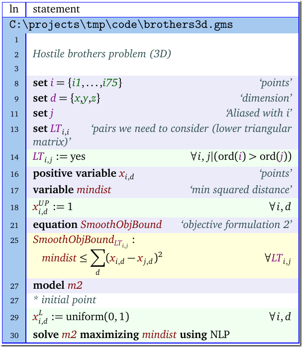
Update: 3d version

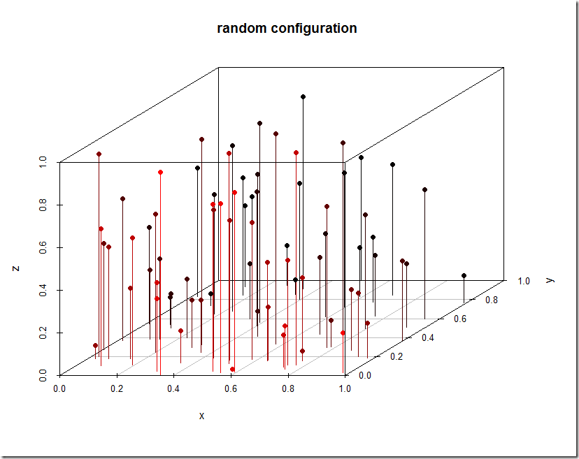
We can generalize to 3d as follows. The plots are somewhat difficult to understand.

image

image image

Note: the red colors are related to the y-coordinate of the point.

Wednesday, January 14, 2015

Pyomo and GAMS

Nice Pyomo introduction: https://www.youtube.com/watch?v=cjMkVHjhSBI

A few small mistakes wrt GAMS:

image

GAMS does not have a complements keyword. Instead it is using a simple notation to match variables to equations in the model statement:

MODEL TRNSP / PROFIT.X, SUPPLY.W, DEMAND.P/ ;

Secondly it is mentioned that GAMS has a presolve facility. Amazingly it does not. It leaves it to the solver to do that. For LP and MIP problems this may be not so bad, although a built-in presolver has some advantages (smaller problems and solutions files to exchange with the solver and most likely better error messages – we have more context available – the importance of this point is often underestimated IMHO). For NLP/MINLP models a built-in presolver can be more important: many nonlinear solvers do not have a presolver built-in. In general a nonlinear presolver is difficult to do inside the solver as the solver doesn’t know the algebraic form – the math – of the nonlinear functions they are executing (of course they can work on the linear part of the model). The most popular NLP solver with GAMS is CONOPT which actually has very good nonlinear presolving facilities (tailored for use with GAMS) and provides excellent diagnostics. But models to be solved with say MINOS or SNOPT can benefit hugely from a presolver (I have seen models being solved much more easily by AMPL with these solvers thanks to the presolving capabilities of AMPL; it really can make a huge difference). Having said this, careful modeling can lead to models where there is little room for the presolver to make a large difference (I try to implement my models this way – I always feel guilty of not doing a good job when the presolver if taking out large chunks of the model. Actually cleaning up a model to get rid of parts that will be presolved away is often a good exercise.).

Sometimes small presolve-like operations need to be performed by GAMS. Often this has to do with the fact that GAMS has an objective variable while solvers have an objective function. For an LP/MIP we would not care (just add an objective row with a single nonzero element at the location of the objective variable). But in case of QPs it is important to substitute out the objective variable (for NLPs this can also be important: linearly constrained problems may be much easier to solve). Even those simple transformation steps are only done in a somewhat half-baked fashion. Here is an LP file for a small QP problem fed into Cplex:

\ENCODING=ISO-8859-1
\Problem name: gamsmodel

Maximize
_obj: zobj + [ 2 z(bin1) ^2 + 2 z(bin2) ^2 + 2 z(bin3) ^2 + 2 z(bin4) ^2
       + 2 z(bin5) ^2 ] / 2
Subject To
objective:         zobj  = 0
bincapacity(bin1): 12 x(job1.bin1) + 11 x(job2.bin1) + 9 x(job3.bin1)
                    + 10 x(job4.bin1) + z(bin1)  = 10
bincapacity(bin2): 12 x(job1.bin2) + 11 x(job2.bin2) + 9 x(job3.bin2)
                    + 10 x(job4.bin2) + z(bin2)  = 12
bincapacity(bin3): 12 x(job1.bin3) + 11 x(job2.bin3) + 9 x(job3.bin3)
                    + 10 x(job4.bin3) + z(bin3)  = 10
bincapacity(bin4): 12 x(job1.bin4) + 11 x(job2.bin4) + 9 x(job3.bin4)
                    + 10 x(job4.bin4) + z(bin4)  = 14
bincapacity(bin5): 12 x(job1.bin5) + 11 x(job2.bin5) + 9 x(job3.bin5)
                    + 10 x(job4.bin5) + z(bin5)  = 16
assign(job1):      x(job1.bin1) + x(job1.bin2) + x(job1.bin3) + x(job1.bin4)
                    + x(job1.bin5)  = 1
assign(job2):      x(job2.bin1) + x(job2.bin2) + x(job2.bin3) + x(job2.bin4)
                    + x(job2.bin5)  = 1
assign(job3):      x(job3.bin1) + x(job3.bin2) + x(job3.bin3) + x(job3.bin4)
                    + x(job3.bin5)  = 1
assign(job4):      x(job4.bin1) + x(job4.bin2) + x(job4.bin3) + x(job4.bin4)
                    + x(job4.bin5)  = 1
Bounds
      zobj Free
0 <= x(job1.bin1) <= 1
0 <= x(job1.bin2) <= 1
0 <= x(job1.bin3) <= 1
0 <= x(job1.bin4) <= 1
0 <= x(job1.bin5) <= 1
0 <= x(job2.bin1) <= 1
0 <= x(job2.bin2) <= 1
0 <= x(job2.bin3) <= 1
0 <= x(job2.bin4) <= 1
0 <= x(job2.bin5) <= 1
0 <= x(job3.bin1) <= 1
0 <= x(job3.bin2) <= 1
0 <= x(job3.bin3) <= 1
0 <= x(job3.bin4) <= 1
0 <= x(job3.bin5) <= 1
0 <= x(job4.bin1) <= 1
0 <= x(job4.bin2) <= 1
0 <= x(job4.bin3) <= 1
0 <= x(job4.bin4) <= 1
0 <= x(job4.bin5) <= 1
Binaries
x(job1.bin1)  x(job1.bin2)  x(job1.bin3)  x(job1.bin4)  x(job1.bin5)
x(job2.bin1)  x(job2.bin2)  x(job2.bin3)  x(job2.bin4)  x(job2.bin5)
x(job3.bin1)  x(job3.bin2)  x(job3.bin3)  x(job3.bin4)  x(job3.bin5)
x(job4.bin1)  x(job4.bin2)  x(job4.bin3)  x(job4.bin4)  x(job4.bin5)
End

Obviously there is some junk left around from what one could say is an incomplete attempt to remove the objective variable. Of course in practice the Cplex presolver will take these parts out.

Friday, January 9, 2015

Scheduling as non-convex MIQP

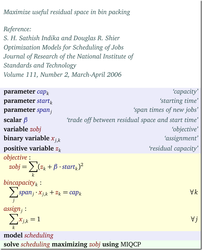
The following model tries to assign jobs to ‘bins’ (bins can be interpreted as workstations) in such a way that the remaining space in the bins is as large as possible (i.e. as little fragmentation as possible so that we have capacity left for large jobs). 

image

Essentially we place high value on large values on remaining capacity zk. We consider here cases with β=0 (if β>0 we also like jobs to be executed early: remaining capacity more in the future is more valuable). This is a non-convex problem so not so easy to solve. This is also the model discussed here.

The choice of a quadratic objective is somewhat arbitrary. It is a simple function that has the required properties that larger values for zk are valued more than proportionally (i.e. linear). In practice I often handle this by some piecewise linear formulation. In addition in practical cases it may be useful to give bins (workstations) without any jobs additional value (no set-up or clean-up in this case, so an unused bin may be preferred). 

With Cplex’s global MIQP solver (http://www.orsj.or.jp/ramp/2014/paper/4-3.pdf) we have now at least three ways to solve this problem with Cplex:(global MIQP, MIP with SOS2 interpolation, MIP with binaries exploiting integer data for capacity and job spans). Using an expanded (larger) version of the dataset provided in the paper with 27 bins and 15 jobs to allocate we try a few formulations.

  • The global MIQP formulation uses the above model directly. We solve to optimality with 4 threads. Cplex selects this algorithm with option SolutionTarget=3.
  • We can add a small value for β to try to reduce some symmetry in the model. We are still aiming for large remaining capacities, but we add a little bit of noise to distinguish similar solutions. The purpose is not really to add a ‘schedule as early as possible’ objective but rather just to increase the performance of the branch-and-bound algorithm. In the experiment we use β=0.01. Note: this may not always give us the same optimal solution.
  • We can use a piecewise linear formulation using SOS2 variables. In this case we used 4 segments. Obviously this is an approximation, so we may arrive at a different optimal solution. However in this case just using 4 segments is good enough to find the global optimum.
  • We can assume all capacity and job length data is integer (as is the case for the example data sets in the paper), and use this to formulate a linear model with extra binary variables. Essentially we implement a table lookup. If all data is integer valued (and the range of the numbers is not outrageously large) this will give us the proven optimal solution of the original MIQP. Exploiting properties of the input data can be key to solve things fast.

Here are the results:

image

These results confirm my experience. I typically use a piecewise linear formulation with just a few segments for this. In most cases I use even fewer than the 4 segments we used here. This seems often to perform reasonably well.

The authors of the original paper did not explore these alternatives but concluded quickly the global MIQP (implemented in Lingo) was too slow and implemented a heuristic. I am not sure if they would have done the same if they saw these results.

Update:

Instead of somewhat more complex formulations suggested in the comments, a simple table look-up using binary variables can be implemented with three constraints having a SOS1 structure:

image

This will make sure we have y=f(x) where x = 0,1,…,n. This is very close to the SOS2 formulation so took me just minutes to implement.

Wednesday, January 7, 2015

DropSolve

IBM has a cloud-based widget: just drop your input files and get a solution file back.

image

http://www-969.ibm.com/software/analytics/docloud/#demo

Saturday, January 3, 2015

Stopping criteria for meta-heuristics

When running a really small non-convex MIQP problem with GAMS+Localsolver I see:

LocalSolver 5.0 (Win64, build 20141120)
Copyright (C) 2014 Innovation 24, Aix-Marseille University, CNRS.
All rights reserved (see Terms and Conditions for details).

Searching for equations that define variables... found 5
Instance:       20 Variables
                 9 Constraints
                82 Expressions
               132 Operands

    time |           iterations |         #infeas
      0s |                    0 |               4
    time |           iterations |       objective
      1s |               583495 | 2.66000000e+002
      2s |              1406684 | 2.66000000e+002
      3s |              2235323 | 2.66000000e+002
      4s |              3073170 | 2.66000000e+002
      . . . . lots of lines with the same objective
    998s |            677978972 | 2.66000000e+002
    999s |            678600000 | 2.66000000e+002
   1000s |            679218601 | 2.66000000e+002

Stopped due to time limit.
Feasible solution found.
Objective Value: 2.66000000e+002

Obviously the default stopping condition (max time = 1000s) is not very good for this case: we are just sitting there for 99.99% 99.9% of the time already at the optimal solution doing nothing useful. (266 is indeed the global optimum). In general these heuristics have no idea how close they are to an optimal solution, and just rely on the user to provide these time or iteration limits. (MIP solvers have this very powerful bounding information where we can say at any moment in time what the gap is between the best solution found an the best solution possible).

Is there nothing better we can do? There is some research on probabilistic stopping rules for these kind of algorithms (i.e. stop as soon as we think the probability we will find a better solution is small):

  • Ribeiro, Rosseti, Souza, “Effective probabilistic stopping rules for randomized metaheuristics: GRASP implementations”, Learning and Intelligent Optimization, Lecture Notes in Computer Science Volume 6683, 2011, pp 146-160
  • Boender, Rinnooy Kan, "Bayesian stopping rules for multistart global optimization methods", Mathematical Programming, 37:59–80, 1987.
  • Dorea, "Stopping rules for a random optimization method", SIAM Journal on Control and Optimization, 28:841–850, 1990.
  • Hart, "Sequential Stopping Rules for Random Optimization Methods with Applications to Multistart Local Search", SIAM Journal on Optimization, 1998, Vol. 9, No. 1 : pp. 270-290
  • Safe, Carballido, Ponzoni, Brignole, “On Stopping Criteria for Genetic Algorithms”, Advances in Artificial Intelligence – SBIA 2004, Lecture Notes in Computer Science, 405-413, 2004

I would guess such a thing could well be a better default stopping rule.

PS Look at these iteration numbers. Don’t care here about a million iterations more or less. (Of course that is the whole purpose of this algorithm: do as many evaluations as possible).